DeepModelingDefine the future of scientific computing together2026-06-21T16:00:00.000Zhttps://blogs.deepmodeling.com/DeepModelingHexoOpen-Source Cloud-Native Alloy Property Calculation Workflow APEX V1.3.0 Released | Toward an Agent-Ready Materials Science Infrastructurehttps://blogs.deepmodeling.com/APEX_2026_06_22/2026-06-21T16:00:00.000Z2026-06-21T16:00:00.000Z
Overview of APEX 1.3.0 Core Upgrades
As a key component of the DeepModeling open-source ecosystem, APEX (Alloy Property Explorer) [1] has undergone continuous iterative optimization since the release of V1.2.0, focusing on high-throughput materials property calculation scenarios. These efforts have steadily enhanced workflow automation, computational efficiency, and user experience, driving the AI for Materials (AI4M) infrastructure toward greater intelligence and standardization.
The newly released APEX V1.3.0 introduces comprehensive upgrades across multiple fronts, including automated structure construction, novel property calculation workflows, a graphical user interface (GUI), and task fault-tolerance with diagnostic mechanisms. This release further reduces manual intervention in complex computational pipelines while improving execution stability and traceability.
More importantly, this upgrade marks a critical step for APEX in evolving from a “computational tool” toward a “scientific agent infrastructure”: automated structure generation, standardized task encapsulation, and workflow composability lay the foundation for building materials computation services that can be directly invoked by AI agents. Whether it is composition-aware structure generation, sublattice-aware random solid-solution construction, or batch task management and multi-workflow tracking within the graphical interface, all these features reflect APEX’s significant progression toward an agent-ready research infrastructure.
Intelligent Structure Generation: Making Materials Structure Construction More Efficient and Smarter
In materials property calculations, structure preparation is often the most fundamental yet time-consuming step. For complex systems, the quality of structure construction directly affects the reliability of subsequent calculations and largely determines the efficiency ceiling of high-throughput studies.
To address this challenge, APEX V1.3.0 has systematically upgraded its structure generation module, significantly enhancing automated construction capabilities. The new version can automatically estimate reasonable lattice parameters based on material composition and, in conjunction with compositional constraints and atomic number requirements, automatically generate supercell structures suitable for various computational scenarios.
For typical ordered structure systems such as B2, L1₂, and L1₀, APEX now supports sublattice-aware random solid-solution generation, combined with Warren–Cowley short-range order parameters to achieve physically more realistic configurational sampling. Meanwhile, the workflow can automatically identify parent lattice information and complete the initialization of complex alloy systems based on prototype structures, substantially lowering the modeling barrier for high-entropy alloys, multi-principal-element alloys, and other complex material systems.
Through these upgrades, APEX can now automatically accomplish the entire pipeline from lattice parameter estimation and supercell construction to complex initial structure generation, providing a more stable and standardized data foundation for high-throughput materials screening and machine-learning interatomic potential training.
Expanding the Boundaries of Materials Property Calculations and Building a More Comprehensive Research Workflow System
After structure automation, the next priority is to cover as many materials property calculation scenarios as possible. However, different material properties often depend on distinct software ecosystems and computational pipelines. Workflow fragmentation, complex parameter configurations, and difficulties in unified result management have persistently constrained high-throughput research.
Addressing this pain point, APEX V1.3.0 further expands its materials property calculation workflow landscape by incorporating several new key property calculation capabilities. In the domain of defect and interface property studies, the new version introduces a Gamma‑Surface workflow that enables automated calculation of the generalized stacking-fault energy surface (γ‑surface). APEX significantly streamlines this process through automated workflows and adds a visual preview function before calculation, allowing users to intuitively inspect the fault-migration path prior to job submission, thereby improving the accuracy and efficiency of computational setups.
Furthermore, the new version supports automatic extraction of Grüneisen parameters and, combined with phonon calculation results under various volumetric strains, enables systematic analysis of thermal expansion behavior. It also implements automated computation of elastic tensors, stress responses, and derived mechanical parameters, making it more convenient for researchers to evaluate materials’ mechanical performance under actual service temperatures. Additionally, the finite-temperature lattice workflow has been optimized, with improved thermodynamic information output, temperature-correlation analysis, and lattice-parameter post-processing, further enhancing the reliability of high-temperature structural stability predictions—particularly beneficial for research on high-temperature structural materials and energy materials.
With the addition of these new workflows, APEX has formed a comprehensive materials property calculation framework covering perfect crystals, defective structures, and finite-temperature systems. This enables systematic investigations from 0 K ground states to real service environments, while also providing richer and higher-quality data sources for high-throughput computations, machine-learning interatomic potential training, and AI-driven materials discovery.
Redefining the Research Interaction Experience: Making Advanced Computational Capabilities Accessible
For a long time, high-performance materials computing platforms, despite their powerful capabilities, have relied heavily on complex command-line operations and tedious parameter configurations. For many non-computational materials science researchers, the real barrier lies not in the scientific questions themselves, but in the learning curve of the toolchain. To this end, APEX V1.3.0 has comprehensively upgraded its graphical user interface (GUI), elevating it from an auxiliary tool to a parallel, important interaction entry point alongside the command-line system, providing a more intuitive and efficient experience for researchers with diverse backgrounds.
The new GUI, built on a browser-based architecture, enables a one-stop process for structure upload, calculation configuration, and job submission. The system automatically identifies the input structure type and generates corresponding configuration templates, eliminating substantial repetitive operations. For mainstream computational software such as VASP and ABACUS, the parameter editing experience has also been specifically optimized, with clearer interface logic and more user-friendly presentation of complex computational workflows. Researchers can quickly launch different types of calculation tasks without manually configuring a large number of parameters in the command line.
As research scales up, batch task management becomes a necessity. V1.3.0 supports one-click submission of large configuration ensembles, unified monitoring of multiple workflows, and cross-task result retrieval, allowing users to grasp the running status of dozens or even hundreds of tasks within a single interface, significantly improving research efficiency. Meanwhile, the synergy between APEX and the Bohrium cloud platform has been further refined, with unified account management and default configuration injection enabling seamless transitions from local development to cloud execution. For data-sensitive scenarios, local resource scheduling remains supported, ensuring that computations can be completed on local clusters without data leaving the secured domain. Result presentation and report management have also become more flexible, closing the loop from submission to result interpretation more smoothly.
Building a More Reliable Research Infrastructure
The real challenge of high-throughput computing often lies in scale: once tasks number in the hundreds, failures, environmental fluctuations, and resource anomalies become almost inevitable. To address this, APEX V1.3.0 has undergone comprehensive optimization around task reliability. The new version enhances workflow failure awareness and diagnostic capabilities, automatically terminating subsequent invalid computations upon critical-step anomalies while recording complete execution statuses and diagnostic information to help researchers quickly pinpoint problem sources. At the same time, the platform improves debugging artifact management, enabling unified tracking and retrieval of computational logs, error messages, and intermediate results, thus providing a more adequate basis for complex issue analysis. Furthermore, the platform introduces intelligent recovery and retry mechanisms that automatically identify different failure causes and execute corresponding strategies, improving resource utilization efficiency while ensuring computational correctness; successfully completed steps are automatically skipped with result reuse, avoiding time and resource consumption from redundant recomputation. These improvements are particularly valuable for long-duration, high-concurrency database construction and high-throughput screening efforts.
Integrating into the Agentic Science Ecosystem and Unleashing the Potential of Scientific Agents
Scientific agents are transitioning from conceptual frameworks to practical deployment. In future research, agents will increasingly undertake literature reading, scheme generation, computation execution, and result analysis [2][3]. This evolution also changes the requirements for computing platforms: they must not only compute fast but also be callable in a standardized manner and reproducibly traceable. APEX’s standardized workflows, unified data interfaces, and cloud-native architecture are precisely laid out in anticipation of this trend.
This capability also creates conditions for deep synergy between APEX and next-generation materials science agent platforms such as MatMaster [4]. MatMaster can discover potential design spaces from vast literature and historical data, generating numerous candidate materials along with corresponding schemes, while APEX provides efficient and reliable property calculation and validation capabilities for these candidates. Together, they establish a closed-loop R&D process of “reading–computing–doing,” dramatically improving materials innovation efficiency. Particularly in application scenarios of machine-learning interatomic potentials—such as high-throughput screening, finite-temperature property prediction, and defect structure evaluation—APEX’s continually expanding workflow capabilities provide high-quality data and validation support for agent-driven materials design. As platform standardization deepens, an increasing number of research tools and agents will be able to collaborate based on a unified infrastructure.
Summary and Outlook
APEX V1.3.0, through automated structure generation, expanded property calculation workflows, a comprehensively upgraded GUI, and robust task management mechanisms, further lowers the barrier to entry for materials property calculations while enhancing the efficiency and reliability of large-scale high-throughput research. Looking ahead, the platform will continue to extend its capabilities in defect structures, finite-temperature methods, and multi-scale simulations, promote deeper integration with mainstream computational software such as Quantum ESPRESSO and GROMACS, and build a more open and comprehensive materials computation ecosystem. Moreover, leveraging the Bohrium and SciMaster ecosystems, APEX will continuously improve its synergy with scientific agents, facilitating efficient coupling among materials design, property prediction, computational validation, and experimental feedback, thereby providing a solid computational infrastructure for the AI for Materials ecosystem.
[2] SciMaster: Towards General-Purpose Scientific AI Agents, Part I. X-Master as Foundation: Can We Lead on Humanity’s Last Exam? https://arxiv.org/abs/2507.05241
[3] Bohrium + SciMaster: Building the Infrastructure and Ecosystem for Agentic Science at Scale. https://arxiv.org/abs/2512.20469
]]><h2 id="Overview-of-APEX-1-3-0-Core-Upgrades"><a href="#Overview-of-APEX-1-3-0-Core-Upgrades" class="headerlink" title="Overview of APEX 1.3.0 Core Upgrades"></a>Overview of APEX 1.3.0 Core Upgrades</h2><p>As a key component of the DeepModeling open-source ecosystem, APEX (Alloy Property Explorer) [1] has undergone continuous iterative optimization since the release of V1.2.0, focusing on high-throughput materials property calculation scenarios. These efforts have steadily enhanced workflow automation, computational efficiency, and user experience, driving the AI for Materials (AI4M) infrastructure toward greater intelligence and standardization.</p>
<p>The newly released APEX V1.3.0 introduces comprehensive upgrades across multiple fronts, including automated structure construction, novel property calculation workflows, a graphical user interface (GUI), and task fault-tolerance with diagnostic mechanisms. This release further reduces manual intervention in complex computational pipelines while improving execution stability and traceability.</p>
<p>More importantly, this upgrade marks a critical step for APEX in evolving from a “computational tool” toward a “scientific agent infrastructure”: automated structure generation, standardized task encapsulation, and workflow composability lay the foundation for building materials computation services that can be directly invoked by AI agents. Whether it is composition-aware structure generation, sublattice-aware random solid-solution construction, or batch task management and multi-workflow tracking within the graphical interface, all these features reflect APEX’s significant progression toward an agent-ready research infrastructure.</p>What Can DP Do too? | Machine Learning Interatomic Potential for Mg-Al-Si-O System Boosts Deep Earth Material Researchhttps://blogs.deepmodeling.com/DeePMD_2026_06_17/2026-06-16T16:00:00.000Z2026-06-16T16:00:00.000Z
Phase diagrams and thermodynamic properties of deep Earth materials are fundamental to geophysics, geodynamics and geological research. As the core chemical system of mantle mineralogy, the Mg-Al-Si-O system governs the stability and physical properties of dominant mantle minerals and melts, further modulating mantle dynamics and plate tectonics. Recently, Xin Zhong, Timm John from Free University of Berlin and Yifan Li from Princeton University published their research A general purposed machine learning interatomic potential for Mg-Al-Si-O system suitable for Earth materials at high pressure and temperature conditions in npj Computational Materials. The team developed a universal machine learning interatomic potential for the Mg-Al-Si-O system. By combining the r2SCAN functional with pairwise Gaussian energy correction, the average enthalpy error of over 20 mineral phases was reduced from 5.2 kJ/mol to 1.2 kJ/mol. The potential reproduces phase diagrams of systems including SiO2 Al2SiO5 and Mg2SiO4 with excellent consistency against experimental measurements. The study quantitatively characterizes the anisotropy of solid–melt interfacial free energy for periclase and forsterite at the atomic scale, and quantifies how non-hydrostatic stress modulates the α-β quartz phase transition.
Research Background
The Mg-Al-Si-O chemical system underpins mantle mineralogy, encompassing major mineral endmembers such as olivine, pyroxene, spinel, garnet and bridgmanite. High-pressure mineral phase transitions account for seismic discontinuities within the Earth’s interior, while accurate phase diagrams rely on precise thermodynamic property data. Although laboratory experiments constrain these properties, atomistic simulations — including molecular simulations with interatomic potentials and density functional theory (DFT) calculations — have emerged as powerful tools for investigating mineral elasticity, surface energy, atomic diffusion and other critical properties. Nevertheless, conventional empirical potentials face severe limitations when modeling large-scale systems and complex phenomena such as phase transitions. Machine learning interatomic potentials trained on high-fidelity DFT datasets, especially those constructed with meta-GGA functionals like SCAN, exhibit exceptional capability to reproduce experimental phase diagrams and thermodynamic observables.
High-Precision Deep Potential Model: A Novel Tool for Earth Material Simulations
This work develops a machine learning interatomic potential for the Mg-Al-Si-O system based on the DeePMD-kit framework. The training dataset covers more than 20 typical rock-forming minerals and their corresponding melts. Initial atomic configurations are primarily sampled from Car–Parrinello molecular dynamics (CPMD) simulations spanning 300–3000 K and 0–50 GPa, supplemented by random structural perturbations of known crystal structures. An active learning strategy analogous to the DP-GEN workflow is adopted to iteratively enhance model robustness and applicable domain via a closed loop: potential training → novel configuration generation → training set augmentation.
The Al2SiO5 polymorph system (kyanite–andalusite–sillimanite) is selected as a benchmark to benchmark the performance of exchange-correlation functionals. This system features tiny energy gaps between distinct mineral phases, rendering it highly sensitive to functional accuracy and thus ideal for validating thermodynamic calculations of geologic materials. Results demonstrate that the r2SCAN functional yields energy errors below 3 kJ/mol for this system, alongside stable self-consistent field convergence, making it well-suited for subsequent melt simulations and training dataset construction.
A core technical advance, pairwise Gaussian energy correction, is implemented to further refine phase stability predictions. This correction scheme introduces subtle adjustments to inter-element interaction energies while preserving the intrinsic accuracy and atomic interaction features of r2SCAN, aligning enthalpy values computed from the machine learning potential with reference thermodynamic databases.
The correction drastically improves the model’s predictive power for mineral phase stability. For over 20 representative mineral phases, the average enthalpy error decreases from 5.2 kJ/mol to 1.2 kJ/mol, with negligible degradation in volume prediction accuracy. This confirms the model retains reliable structural descriptions while achieving drastically improved thermodynamic precision.
(See Figure 1 for the full potential construction workflow; Figure 2 for the performance of Gaussian energy correction.)
Figure 1 Workflow of machine learning potential development and application. The upper panel illustrates initial dataset generation, neural network training, active learning dataset expansion and Gaussian energy correction. The lower panel lists downstream applications enabled by this potential, including molecular dynamics, thermodynamic integration, Monte Carlo/cluster expansion and enhanced sampling simulations.
Figure 2 Functional benchmarking and performance of Gaussian energy correction. The upper subplot compares relative energy errors of different functionals for the Al2SiO5 system. The lower subplot shows marked reductions in enthalpy errors for all mineral phases after correction, with the average error lowered from ~5.2 kJ/mol to ~1.2 kJ/mol.
Phase Diagram Construction: Validation of Model Predictive Capacity
Equipped with the trained machine learning potential and the DPTI package developed by the DeepModeling community, the authors constructed phase diagrams for SiO2 , Al2SiO5 and Mg2SiO4. Gibbs free energies are evaluated via thermodynamic integration, and phase boundaries are located using the Clausius–Clapeyron relation, yielding predictions consistent with experimental constraints. (See Figure 3.)
For the SiO2 system, machine learning potential molecular dynamics predicts the stishovite-to-CaCl₂-type post-stishovite transition at ~53 GPa, close to the experimental value of ~60 GPa, verifying the model’s extrapolation capability. The andalusite–sillimanite phase boundary for Al2SiO5 is significantly refined after Gaussian energy correction; Monte Carlo simulations accounting for Al–Si order–disorder effects within sillimanite resolve discrepancies in P–T boundary slopes. For the Mg2SiO4 system, the potential successfully reproduces key features including forsterite melting and the bridgmanite–periclase liquidus. The authors also discuss model limitations: for instance, the ~7 GPa deviation in ultrahigh-pressure SiO2 corresponds to a depth offset of ~200 km, requiring caution when interpreting geophysical observations.
Figure 3 Phase diagrams computed using the machine learning potential. Colored regions denote model predictions, while dashed lines represent experimental or published thermodynamic constraints. The figure presents P-T phase diagrams for SiO2 , Al2SiO5 and Mg2SiO4, alongside the T-X phase diagram of the binary MgO-SiO2 system at 24 GPa.
Order–Disorder Transitions: Atomistic Insight into Sillimanite Thermodynamics
A critical feature of the Al2SiO5 system is Al-Si order–disorder within sillimanite. At elevated temperatures, Al and Si cations rearrange along chain-like structural units, modifying mixing free energy and shifting phase boundary slopes.
The machine learning potential enables efficient energy evaluation for diverse Al-Si atomic arrangements, whose mixing free energies are subsequently quantified via cluster expansion and Monte Carlo simulations. Long-range ordering rapidly decays above ~1300 K, whereas short-range ordering diminishes more gradually, indicating localized intra-chain Al-O-Si coordination persists at higher temperatures. Compared with the conventional Bragg-Williams approximation, this atomistic framework predicts mixing free energies ~25% lower, delivering refined atomic-scale constraints on sillimanite stability.
Solid–Melt Interfacial Free Energy: A Hard-to-Measure Experimental Observable
Beyond phase diagram modeling, the study calculates solid–melt interfacial free energy, a parameter inaccessible to routine laboratory characterization. This quantity governs crystal morphology, melting mechanisms, melt distribution along grain boundaries, and microstructural evolution of high-temperature mantle materials.
The computational workflow is summarized as follows: periodic supercells with coexisting solid and molten domains are constructed, and free energy profiles are obtained via umbrella sampling and metadynamics. At the melting point, the Gibbs free energy difference between a pure solid cell and a solid–melt coexistence cell arises from two solid–melt interfaces formed under periodic boundary conditions. Dividing this free energy difference by twice the interfacial area yields the solid–melt interfacial free energy.
For periclase at 24 GPa and 5200 K, metadynamics and umbrella sampling deliver consistent interfacial free energy values ranging from 0.62 to 0.66 J/m², with an interfacial anisotropy of ~ 6%. For structurally complex forsterite, metadynamics exhibits slow convergence, so umbrella sampling with chemical potential correction is adopted. Results show the (010) plane bears the lowest interfacial free energy (~ 0.29 J/m²), while the (001) plane exhibits the highest value (~ 0.33 J/m²), corresponding to an anisotropy of ~12%. Such anisotropic information cannot be directly resolved by existing experimental techniques.
Figure 4 Calculation of solid–melt interfacial free energy. The upper subplot presents periclase–melt interfaces, showing consistent outputs from metadynamics (MetaD) and umbrella sampling (US). The lower subplot displays forsterite–melt interfacial free energies for distinct crystallographic planes, revealing ~12% anisotropy.
Non-Hydrostatic Stress Effects: New Perspective on the α-β Quartz Transition
The α-β quartz transition, driven by rotation of Si-O-Si bond angles, serves as an ideal model system to probe non-hydrostatic stress effects. Simulations at 1200 K with variable differential stress track Si-O-Si bond angle evolution as a function of mean stress. The results indicate that each 1 GPa increment in differential stress shifts the mean transition stress by ~0.17 GPa, introducing up to 17% systematic error if mean stress alone is used as the transition criterion.
Under typical crustal conditions, differential stress within quartzite commonly ranges from 0.1 to 0.3 GPa, inducing a transition pressure offset of merely 0.02–0.06 GPa, equivalent to negligible depth shifts. Therefore, non-hydrostatic stress will not drastically alter the P–T stability window of the α-β quartz transition unless extreme localized differential stress occurs.
Conclusions and Outlook
This research delivers more than a standalone Deep Potential interatomic potential; it establishes a complete, standardized workflow for computational modeling of Earth materials: appropriate DFT functionals guarantee accurate structural and energetic descriptions, active learning expands the sampled configuration space, thermodynamic database-based energy correction refines phase stability predictions, and cross-validation against experimental phase diagrams validates overall model reliability.
The resulting machine learning potential enables investigations intractable for conventional experiments or ab initio calculations, including high-P/T solid–melt interfacial free energies, order–disorder mixing free energies, stress-modulated phase transition pathways, and future simulations of complex multi-component mantle lithologies. Although the current potential only covers the four-component Mg-Al-Si-O system, this work lays a solid foundation for extensions toward multi-element solid solutions and compositional models representative of natural rock assemblages.
]]><p>Phase diagrams and thermodynamic properties of deep Earth materials are fundamental to geophysics, geodynamics and geological research. As the core chemical system of mantle mineralogy, the Mg-Al-Si-O system governs the stability and physical properties of dominant mantle minerals and melts, further modulating mantle dynamics and plate tectonics. Recently, Xin Zhong, Timm John from Free University of Berlin and Yifan Li from Princeton University published their research A general purposed machine learning interatomic potential for Mg-Al-Si-O system suitable for Earth materials at high pressure and temperature conditions in npj Computational Materials. The team developed a universal machine learning interatomic potential for the Mg-Al-Si-O system. By combining the r2SCAN functional with pairwise Gaussian energy correction, the average enthalpy error of over 20 mineral phases was reduced from 5.2 kJ/mol to 1.2 kJ/mol. The potential reproduces phase diagrams of systems including SiO<sub>2</sub> Al<sub>2</sub>SiO<sub>5</sub> and Mg<sub>2</sub>SiO<sub>4</sub> with excellent consistency against experimental measurements. The study quantitatively characterizes the anisotropy of solid–melt interfacial free energy for periclase and forsterite at the atomic scale, and quantifies how non-hydrostatic stress modulates the α-β quartz phase transition.</p>What Can DP Do too? | Large Atomic Model DPA2 Enables Cross-Scale Simulations of Complex Nuclear Alloyshttps://blogs.deepmodeling.com/DeePMD_2026_05_29/2026-05-28T16:00:00.000Z2026-05-28T16:00:00.000Z
Next-generation nuclear fission and fusion reactors impose extremely stringent requirements on structural materials, which must simultaneously withstand high temperatures, high-dose irradiation, and strongly corrosive coolants. Multi-principal element alloys (MPEAs) are regarded as highly promising candidate materials owing to their unique high-entropy effect, lattice distortion, sluggish diffusion, and cocktail effect. Nevertheless, understanding irradiation damage and mechanical behaviors at the atomic scale in these complex alloys demands interatomic potentials (IAPs) with high precision and universal transferability. Although conventional machine learning interatomic potentials (MLIAPs) achieve decent accuracy, the volume of training datasets rises exponentially for quinary or higher-order complex systems, leading to prohibitive computational costs for generating DFT reference labels.
Recently, the research group led by Biao Xu and Huiqiu Deng from Hunan University, together with Chih-Chung Kai from City University of Hong Kong, published the paper Scaling reliable interatomic potentials to complex nuclear alloys via pretrained atomic models in npj Computational Materials. For the first time, the study integrates multi-task physics-informed pretraining with Large Atomic Models (LAMs), and systematically evaluates the performance of IAP construction for the complex nuclear alloy Ta-Nb-W-Mo-V. The DPA2-5E model fine-tuned merely with quinary alloy data not only outperforms conventionally trained MLIAPs built from scratch, but also exhibits robust transferability toward quaternary, ternary, and even binary subsystems. It faithfully reproduces irradiation cascade damage and stress-strain responses.
Dataset and Model Training Strategy: Balancing Structural Diversity and Computational Cost
This study adopts the public dataset of the Ta-Nb-W-Mo-V quinary alloy and all its 30 subsystems spanning unary to quaternary compositions, covering 31 alloy systems in total. The dataset encompasses crystalline configurations with vacancies and interstitials, free surfaces, liquid phases, chemically ordered phases, and transition-state geometries, ensuring full coverage of the configuration space (see Figure 1).
Based on this fixed, representative dataset, the authors systematically compare two training paradigms:
Fine-tuning the pre-trained large atomic model DPA2: DPA2-5E trained only on quinary alloy data, and DPA2-All trained on all 31 alloy systems.
Training the baseline DPA1 model from scratch: DPA1-5E trained only on quinary alloy data, and DPA1-All trained on the full dataset.
Figure 1 Schematic of the diverse training dataset encompassing the Ta-Nb-W-Mo-V quinary alloy and all its subsystems. Colored circles represent the five constituent elements (W, Ta, Nb, Mo, and V). The colored lines and closed loops connecting or enclosing multiple circles denote alloy subsystems formed by corresponding element combinations. (a) Five unary (single-element) systems; (b) 10 binary combinations; (c) 10 ternary combinations; (d) five quaternary combinations; (e) one quinary system, forming 31 alloy systems in total.
The detailed training workflow is illustrated in Figure 2. The DPA2 model is fine-tuned from the multi-task pretrained checkpoint (DPA2_medium_28_10M_rc0.pt), and knowledge distillation is implemented to generate a lightweight student model for higher computational efficiency. By contrast, the DPA1 model is trained from scratch with identical attention descriptors and neural network architectures.
Figure 2 Schematic illustration of the model training workflows. (a) Conversion of dataset formats. (b) Fine-tuning and knowledge distillation procedure for the LAM-based DPA2 model. (c) Training pipeline of the DPA1 baseline model.
Model Accuracy and Transferability: Outstanding Performance under Low-Data Regimes
When trained on the full Dataset-All, DPA2-All achieves lower global root-mean-square errors (RMSEs) for energy and force than DPA1-All and the tabGAP-All potential reported in existing literature. More importantly, under the low-data scenario where only quinary alloy data is used for training, the validation energy and force RMSEs of DPA2-5E are markedly superior to those of DPA1-5E (Figure 3c,d). This result demonstrates that the physical prior knowledge embedded in the multi-task pre-trained large model effectively improves model robustness and generalization even with limited training data.
Figure 3 Energy and force prediction performance of five MLIAPs built from different datasets (Dataset-All includes all quinary down to unary data) and training strategies. (a, b) Training errors of five MLIAPs on different datasets. (c, d) Validation errors of five MLIAPs on different datasets. Dark-blue filled circles: DPA2-All; light-blue filled circles: DPA2-5E; dark-orange filled circles: DPA1-All; light-orange filled circles: DPA1-5E; open blue star: reference tabGAP-All potential. Solid lines serve as visual guides.
The study further quantifies the downward transferability of the potentials. DPA2-5E, which is exclusively trained on quinary alloy data, yields prediction errors for quaternary and ternary subsystems nearly equivalent to those of DPA2-All, revealing excellent cross-component transferability. Although DPA1-5E retains moderate transferability, its prediction accuracy degrades far more drastically when extended to lower-order subsystems. This indicates that both model architecture and pretrained physical priors jointly govern transfer performance. This "one model for multiple systems" paradigm drastically cuts the cost of developing individual potentials for each alloy composition.
Irradiation Cascade Simulations: Faithful Reproduction of Defect Evolution
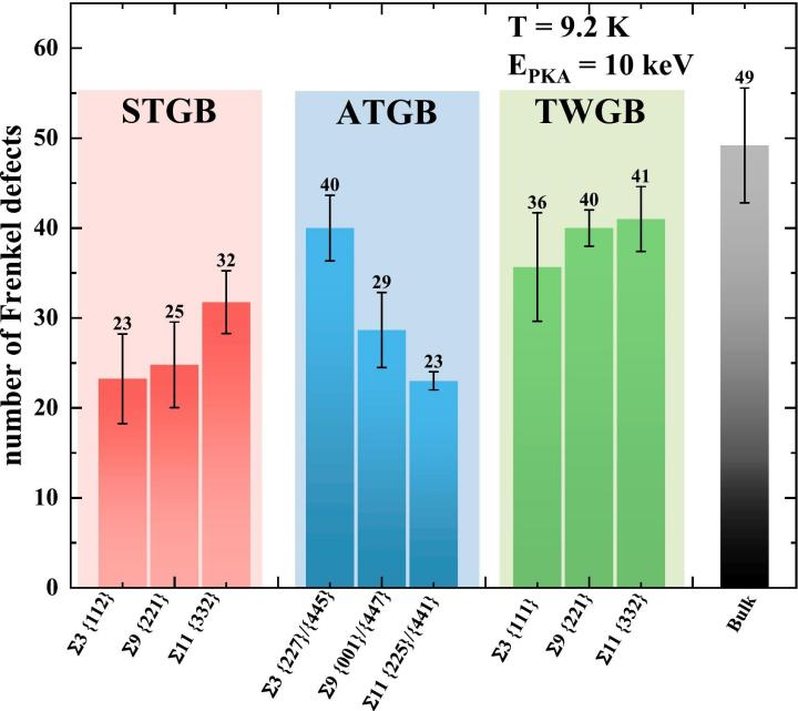
Displacement cascade simulations are performed at 300 K with primary knock-on atom (PKA) energies ranging from 2 keV to 10 keV to compare the predictive power of DPA2-5E and the high-fidelity reference model DPA2-All. For the quinary Ta-Nb-W-Mo-V alloy, quaternary Ta-Nb-W-Mo alloy, and binary Ta-W alloy, the two potentials produce nearly identical numbers of Frenkel pairs at the thermal spike stage and after structural relaxation. No statistically significant discrepancy is observed in the elemental distribution of interstitial defects (Figure 4). It proves that DPA2-5E trained solely on the quinary alloy can precisely capture irradiation damage behaviors, even for untrained lower-order subsystems.
Figure 4 Primary radiation damage outcomes predicted by DPA2-All and DPA2-5E trained only on the quinary alloy dataset. Scatter points denote the number of Frenkel pairs formed at the thermal spike, while bars represent Frenkel pair populations after thermal equilibration at 300 K, plotted against PKA energy for (a) quinary Ta-Nb-W-Mo-V, (b) quaternary Ta-Nb-W-Mo, and (c) binary Ta-W alloys. Red symbols/bars: DPA2-All; blue symbols/bars: DPA2-5E. Error bars represent the standard deviation calculated from 20 independent cascade simulations. Elemental composition of interstitial atoms after relaxation following 10 keV cascades for (d) Ta-Nb-W-Mo-V, (e) Ta-Nb-W-Mo, and (f) Ta-W alloys. Each stacked bar differentiates interstitial fractions of constituent elements (V, Nb, Mo, Ta, W) with distinct color coding.
Mechanical Property Prediction: Temperature Dependence and Systematic Softening
The DPA2-5E potential predicts the temperature-dependent decline of compressive yield strength for Ta-Nb-W-Mo-V, Ta-Nb-W-Mo, and Ta-W alloys, showing excellent consistency with DPA2-All (Figure 5). Quantitatively, DPA2-5E slightly underestimates yield strength, corresponding to systematic softening, and the prediction bias gradually increases when extending from the parent quinary composition to binary subsystems. The authors note that incorporating non-equilibrium structural configurations into the fine-tuning dataset can partially mitigate this issue, yet the improvement remains limited for compositions far from the training quinary alloy. This observation pinpoints the inherent limitation arising from the near-equilibrium bias of the pretraining dataset, and provides clear directions for future optimization.
Figure 5 Temperature dependence of compressive yield strength for the parent alloy and its subsystems predicted by LAM-based MLIAPs. Compressive yield strength versus temperature for equimolar Ta-Nb-W-Mo-V, Ta-Nb-W-Mo, and Ta-W alloys, calculated by DPA2-5E and the reference DPA2-All: (a) Ta-Nb-W-Mo-V, (b) Ta-Nb-W-Mo, (c) Ta-W. Blue solid lines: DPA2-All; orange solid lines: DPA2-5E. Yellow markers with vertical error bars denote the mean value and one standard deviation over 10 parallel simulations.
Extended Applications: Complex Microstructures and Corrosive Environments
This framework is not restricted to compositionally complex single-phase alloys. The method is further validated on ordered intermetallics (dual-phase FCC + L1₂ structure in the Ni-Co-Fe-Cr-Al-Ti-Ta system) and a six-component L1₂ alloy exposed to liquid lead-bismuth corrosion with and without oxygen contamination. Even under such extreme structural and environmental complexity, the MLIAP built upon the pretrained LAM achieves high prediction accuracy with minimal additional training data (Figure 6), which verifies the generalizability of this approach.
Figure 6 Energy and force prediction errors of MLIAPs developed via the pretrained LAM strategy for three representative complex systems. The "L1₂-6 + PbBi + O" system consists of solid L1₂-6 precipitates (Ni, Co)₃(Al, Ti, Ta, Nb), surrounding liquid Pb-Bi phase, and oxide phases. The "FCC + L1₂-7" system contains a disordered FCC matrix (Ni-Co-Fe-Cr-Al-Ti-Ta) and coherent L1₂ precipitates (Ni, Co)₃(Fe, Cr, Al, Ti, Ta). Orange bars: training RMSE; green bars: validation RMSE. (a) Energy prediction RMSE; (b) force prediction RMSE.
Summary
This work pioneers the application of the multi-task pretrained Large Atomic Model DPA2 in developing interatomic potentials for nuclear structural alloys. The DPA2-5E model fine-tuned only on quinary alloy data strikes an excellent balance among prediction accuracy, cross-component transferability, and computational cost. The potential faithfully reproduces irradiation-induced defect evolution and temperature-dependent mechanical responses, and can be reliably extended to quaternary down to unary subsystems. Moreover, the workflow is adaptable to dual-phase microstructures and material systems under corrosive conditions.
This hierarchical "one model for multiple systems" workflow offers a practical and scalable route for high-throughput screening of complex nuclear materials, cross-comparison among alloy compositions, and long-term atomic-scale damage evolution simulations.
All datasets and training scripts are publicly available at:https://github.com/JiangXiaoMingSan/LAM-DPA-Train-Script
]]><p>Next-generation nuclear fission and fusion reactors impose extremely stringent requirements on structural materials, which must simultaneously withstand high temperatures, high-dose irradiation, and strongly corrosive coolants. Multi-principal element alloys (MPEAs) are regarded as highly promising candidate materials owing to their unique high-entropy effect, lattice distortion, sluggish diffusion, and cocktail effect. Nevertheless, understanding irradiation damage and mechanical behaviors at the atomic scale in these complex alloys demands interatomic potentials (IAPs) with high precision and universal transferability. Although conventional machine learning interatomic potentials (MLIAPs) achieve decent accuracy, the volume of training datasets rises exponentially for quinary or higher-order complex systems, leading to prohibitive computational costs for generating DFT reference labels.</p>DPA4 Tops Matbench Discovery: A Single RTX 5090 Delivers SOTA-Level Large Atomic Models in One Dayhttps://blogs.deepmodeling.com/DPA4_05_22_2026/2026-05-21T16:00:00.000Z2026-05-21T16:00:00.000Z
Recently, the OpenLAM Team of the AI fof Science Institute,Beijing(AISI), Peking University, DP Technology, and the Institute of Applied Physics and Computational Mathematics have jointly launched DPA4, a new-generation model architecture tailored for the era of Large Atomic Models (LAMs). DPA4 claimed the top spot worldwide with its comprehensive performance score (CPS) on Matbench Discovery, an authoritative global benchmark for materials discovery, emerging as the latest State-of-the-Art (SOTA) model.
DPA4’s highlight lies in its ultra-low training threshold: the prior leading eSEN needed over 300 GPU days for training, yet DPA4 reaches matching accuracy with merely one consumer RTX 5090 running for roughly one day, and its parameter volume is less than one-tenth of eSEN’s.
In short, the SOTA-level accuracy once reliant on costly supercomputing is now accessible via a single consumer graphics card. DPA4 reshapes the accuracy-efficiency Pareto frontier of large atomic models.
Official Screenshot of Matbench Discovery (Data as of May 22, 2026)
DPA4 adopts SO(2) equivariant linear operators paired with local-coordinate attention. It satisfies translation, rotation, permutation symmetries and energy conservation while cutting equivariant computation costs drastically. It also pioneers global compile-accelerated training for machine learning potentials, lifting training speed 2–3 times. It secured SOTA top rankings on two key benchmarks: Matbench Discovery and SPICE-MACE-OFF. It strikes a new balance of precision and training cost: a single RTX 5090 trains it in one day to match eSEN’s 300+ GPU-day accuracy; parameters are under 1/10 of eSEN; versus its predecessor DPA3, training efficiency is about 10x higher at equal accuracy.
DPA4 early access is open to the DeepModeling community. Its research paper and full official code will be open-sourced later; readers may join the article’s ending WeChat group for academic exchanges. Below is a condensed technical introduction.
1. DPA4 Model Architecture: SO(2) Equivariant Design in Local Coordinate Systems
Traditionally, SO(3) equivariant models rely on complex Clebsch–Gordan tensor products to retain rotational symmetry, whose computational complexity spikes sharply [about O(l6max)] with the increase of angular momentum order lmax— this is the core reason high-precision models demand massive computing resources.
DPA4’s core idea avoids expensive global SO(3) tensor calculations by simplifying symmetry processing to the SO(2) subgroup: it builds a local coordinate frame for each atomic bond, unifying bond orientations to a reference axis. Axial rotation symmetry only requires SO(2) processing, whose simple block-structured linear mappings replace heavy SO(3) tensor operations. Full rotational equivariance is preserved while angular computation overhead drops greatly.
On this basis, DPA4 further incorporates attention mechanisms to aggregate information from neighboring atoms. The model can adaptively focus on the most critical atomic interactions for the central atom according to local geometric and chemical environments, thus delivering strong expressive power with a compact parameter scale. The entire model strictly adheres to translation, rotation, permutation symmetries and energy conservation, ensuring full physical consistency.
Two major engineering optimizations further lift efficiency:
Native torch.compile compatibility: end-to-end acceleration without extra code edits
Embedded ZBL short-range repulsive potential: stabilizes simulations under high pressure, irradiation, defects and other extreme atomic configurations
DPA4 Model Structure Diagram
2. Benchmark Performance: Dual No.1 Titles
Matbench Discovery: Global Champion for Materials Discovery. Launched by UC Berkeley, Cambridge University and other top institutes, Matbench Discovery is the world’s leading dynamic benchmark for AI inorganic material prediction, widely accepted as the industry gold standard. Instead of static data fitting, it tests model capacity to forecast stability of hundreds of thousands of unknown crystals, mimicking real exploratory research. Final Comprehensive Performance Score (CPS) integrates energy/force accuracy, F1 score and discovery acceleration factors. Beating SOTA models from Meta, Microsoft and global universities, DPA4 claimed the top CPS rank.
SPICE-MACE-OFF: Top Small-Molecule Performance. DPA4 excels beyond inorganic crystals, setting a new SOTA record on the SPICE-MACE-OFF small-molecule benchmark. With smaller parameter size, it outperformed the former leading model eSEN to take the first place, proving its versatility as a universal potential energy surface model for crystals and organic small molecules alike.
Performance on SPICE-MACE-OFF
3. Efficiency Breakthrough: A New Precision-Cost Pareto Frontier
Top benchmark results confirm DPA4’s outstanding accuracy, yet its revolutionary value lies in minimal training cost. Conventional leading models always require larger parameters and heavier computation; DPA4 breaks this norm:
Training cost: 1 RTX 5090 (~1 day) = eSEN’s 300+ GPU days of precision
Parameter scale: <1/10 of eSEN at equivalent CPS
Generation upgrade: ~10× training efficiency vs DPA3 under equal prediction accuracy
DPA4 Redefining the Accuracy-Efficiency Pareto Frontier for Large Atomic Models
Multi-layer engineering optimizations enable such efficiency gains. Unlike standard AI models, potential training needs double backward calculation for force derivation, which long blocked torch.compile use and forced large batch sizes to boost GPU utilization. DPA4 is the world’s first machine learning potential supporting compile training. Paired with bf16 automatic mixed precision (AMP), it slashes VRAM usage drastically, enabling full training on a single graphics card.
Comparison of Training Time and Peak Video Memory Usage with DPA4’s Compile and AMP Enabled
This breakthrough accelerates model iteration for researchers; fixed computing budgets support larger-scale, longer-time microscopic simulations. DPA4 turns high-throughput atomic simulation from a high-cost luxury into accessible tools, supporting battery material R&D, catalyst design, semiconductor screening and other key industries.
Summary
DPA4 is a universal next-gen potential framework for the LAM era. Its local SO(2) equivariant operators plus attention maintain physical consistency while cutting computation costs; native compile acceleration and built-in ZBL potential further boost engineering performance.
It claimed dual top benchmark rankings, delivering matching or superior precision to prior costly large models with <1/10 parameters and one-day single-GPU training. DPA4 verifies high accuracy and high efficiency can be achieved simultaneously.
Early access is open to DeepModeling community members; papers and full open-source code will be released sequentially later. The team sticks to open collaboration in LAM research, inviting global scholars to follow progress and join the community.
Core Developers & Affiliated Institutions
Li Tiancheng (Peking University, AISI) Xue Jianming (Peking University) Zhang Linfeng (DP Technology, AISI) Zhang Duo (Peking University, AISI) Wang Han (Institute of Applied Physics and Computational Mathematics)
]]><p>Recently, the OpenLAM Team of the AI fof Science Institute,Beijing(AISI), Peking University, DP Technology, and the Institute of Applied Physics and Computational Mathematics have jointly launched DPA4, a new-generation model architecture tailored for the era of Large Atomic Models (LAMs). DPA4 claimed the top spot worldwide with its comprehensive performance score (CPS) on Matbench Discovery, an authoritative global benchmark for materials discovery, emerging as the latest State-of-the-Art (SOTA) model.</p>
<p>DPA4’s highlight lies in its ultra-low training threshold: the prior leading eSEN needed over 300 GPU days for training, yet DPA4 reaches matching accuracy with merely one consumer RTX 5090 running for roughly one day, and its parameter volume is less than one-tenth of eSEN’s.</p>
<p>In short, the SOTA-level accuracy once reliant on costly supercomputing is now accessible via a single consumer graphics card. DPA4 reshapes the accuracy-efficiency Pareto frontier of large atomic models.</p>
<center><img data-src=https://dp-public.oss-cn-beijing.aliyuncs.com/community/Blog%20Files/DPA4_05_22_2026/DPA41.PNG pic_center width="60%" height="60%" /></center>
<h6 id="Official-Screenshot-of-Matbench-Discovery-Data-as-of-May-22-2026"><a href="#Official-Screenshot-of-Matbench-Discovery-Data-as-of-May-22-2026" class="headerlink" title="Official Screenshot of Matbench Discovery (Data as of May 22, 2026)"></a><em>Official Screenshot of Matbench Discovery (Data as of May 22, 2026)</em></h6>What Can DP Do Too? | Deep Potential Reveals Cerium Segregation and Strengthening Mechanisms in Nanocrystalline Al-Ce Alloyshttps://blogs.deepmodeling.com/DeePMD_2026_05_20/2026-05-19T16:00:00.000Z2026-05-19T16:00:00.000Z
A research team led by Dr. Xue Hongtao and Dr. Chang Zhen from State Key Laboratory of Advanced Processing and Recycling of Non-ferrous Metals & Gansu Center for Materials Genome and Fundamental Structural Research, Lanzhou University of Technology, has published new findings in Journal of Materials Research and Technology. The paper titled Deep potential driven molecular dynamics simulations on tensile properties of nano-grained Al–Ce alloys: Mechanisms of Ce segregation and strengthening develops a high-precision deep potential (DP) for Al-Ce alloys and clarifies the microscale strengthening mechanism induced by grain boundary segregation of trace rare earth cerium (Ce) in nanocrystalline aluminum alloys.
Research Background
Molecular dynamics (MD) is a powerful atomistic simulation method, whose accuracy relies heavily on interatomic potentials. Ab initio molecular dynamics (AIMD) delivers high precision but suffers from exorbitant computational costs, limiting its application to small systems and short time scales. Deep potential (DP) effectively addresses this issue by achieving DFT-level accuracy at low computational overhead, enabling simulations of larger systems over longer durations.
Machine learning potentials have been widely adopted for various metals. However, due to the complex 4f electronic behavior of Ce, reliable potentials for rare-earth doped aluminum alloys (especially Al-Ce systems) remain scarce. Most existing studies focus on phase stability and thermodynamics, while systematic simulations on grain boundary segregation, dislocation motion and large-strain deformation in polycrystalline Al-Ce alloys are insufficient. Therefore, a high-fidelity DP model is urgently required to explore the strengthening mechanism of Ce-doped aluminum.
High-precision DP model: Enabling atomistic simulation of Al-Ce systems
The team adopted the DP-GEN active learning workflow to build the DP model for Al-Ce alloys, supporting atomistic analysis on the alloy’s tensile behaviors. Optimized thoroughly, this model accurately reproduces fundamental physical properties calculated via DFT, including energy-volume curves, equilibrium lattice parameters and elastic constants.
Figure 1: Flowchart of the development and application of machine learning potentials
Table 1: Equilibrium lattice constants (Å) of Al–Ce intermetallic phases (Al₁₁Ce₃, Al₃Ce, and Al₂Ce) obtained via DFT, DP and published literature
As shown in Table 1, the DP model predicts equilibrium lattice constants of Al₁₁Ce₃, Al₃Ce, Al₂Ce and other intermetallic phases with deviations below 1% compared with DFT results. Its predictions for elastic constants are also reliable, with most individual elastic constants deviating within 15%. The DP model also captures phase transition trends consistent with experimental observations. DP-based MD simulations show that the energy curves of α-Al₁₁Ce₃ and β-Al₁₁Ce₃ intersect at around 1300 K, which matches the experimental solid-state α→β phase transition temperature of 1279 K.
Figure 2: Temperature dependence of total energy and volume for Al₁₁Ce₃ polymorphs from DP-based molecular dynamics: (a) total energy-temperature curves of α-Al₁₁Ce₃ and β-Al₁₁Ce₃, (b) volume-temperature curve of β-Al₁₁Ce₃
Cerium segregation behavior: atomic-scale insights into grain boundary engineering
The researchers constructed nanocrystalline Al-Ce models with varying Ce atomic fractions (0, 0.010, 0.0154, 0.0195, 0.021, 0.027 at.%). Using a combined Monte Carlo (MC) and MD annealing scheme, they confirmed that Ce atoms tend to segregate and accumulate at grain boundaries.
Figure 3: Atomic configurations of the Al–Ce models: (a) 3D view, (b) front view. Green: FCC grains; gray/red: grain boundaries and defects
After MC/MD annealing, the relative increase of Ce concentration at grain boundaries for samples with 0.010–0.027 at.% Ce is 27.65%, 85.01%, 3.84%, 36.33% and 13.84% respectively. The minimum increment occurs at 0.0195 at.% Ce, corresponding to the peak yield strength of the alloy.
Figure 4: Fraction of Ce atoms at grain boundaries for different Ce contents, before and after MC equilibration at 300 K
Tensile Properties: Non-monotonic Variation Rule
All samples exhibit typical tensile characteristics of nanocrystalline metals, including a linear elastic stage, peak stress and plastic deformation with random fluctuations. Plastic deformation is mainly governed by dislocation movement and grain boundary sliding.
The yield strength presents a non-monotonic trend with rising Ce content (increasing first and then decreasing). All Al-Ce alloys possess higher yield strength than pure Al. Samples treated with MC/MD annealing always show better mechanical performance than those without annealing. For the 0.0195 at.% Ce sample, the yield strength rises from 1.846 GPa (without MC annealing) to 1.892 GPa (with MC annealing), a 2.5% improvement.
Figure 5: Tensile response of nanocrystalline Al–Ce alloys at different Ce contents: (a) stress-strain curves with MC/MD annealing; (b) stress-strain curves without MC annealing; (c) yield strength vs. Ce content
Strengthening Mechanism: Synergy of Dislocations and Stacking Faults
From 0.010 at.% to 0.0195 at.% Ce, the dislocation density near the yield point and the number of HCP-structured atoms gradually increase, followed by a decline at 0.027 at.% Ce. This variation is highly consistent with the trend of yield strength.
Figure 6: Dislocation density and HCP atoms of nanocrystalline Al–Ce alloys with different Ce contents: (a) dislocation density, (b) number of HCP atoms
At zero strain, dislocations are primarily distributed at grain boundaries and adjacent regions. Samples with higher yield strength have higher initial dislocation density at grain boundaries. For the 0.0195 at.% Ce sample, prominent activation of grain boundary dislocations and intensive dislocation interaction/tangling inside grains are observed.
Figure 7: Dislocation networks in nanocrystalline Al–Ce alloys with different Ce contents: initial configurations at zero strain and configurations at the onset of yielding
Stacking faults preferentially nucleate at grain boundaries and triple junctions and then extend into grain interiors. At a tensile strain of approximately 10%, red HCP atoms emerge around grain boundaries and triple junctions, forming local stacking faults. As the strain increases to 18%–22%, stacking fault bands grow in quantity and length and interact with the grain boundary network.
Figure 8: Atomic snapshots of polycrystalline Al–Ce alloys with different Ce contents at selected tensile strains. Green: FCC grain interiors; gray: grain boundaries; red: HCP atoms
Conclusions and Outlook
Based on the high-precision DP model, this study systematically reveals the roles of Ce segregation and MC/MD annealing in strengthening nanocrystalline Al-Ce alloys. The yield strength reaches the maximum at 0.0195 at.% Ce, which is close to the commonly reported experimental value (~0.02 at.%) with a relative deviation of merely 2.5%. Compared with pure Al, the peak yield strength increases by 7.51%.
These findings deepen the understanding of the strengthening behavior of Al-Ce alloys and provide valuable theoretical guidance for the design and fabrication of high-performance aluminum alloy materials.
References
[1] Chang Z, Feng L, Xue HT, et al. Deep-learning potential molecular dynamics study on nanopolycrystalline Al-Er alloys: effects of Er concentration, grain boundary segregation, and grain size on plastic deformation. Journal of Chemical Information and Modeling, 2024;64:3282-93. https://doi.org/10.1021/acs.jcim.4c00008
[2] Xue HT, Chang Z, Li J, et al. Molecular dynamics simulations of the shear and tensile mechanical properties of rare-earth metal erbium based on deep-learning potential. Materials Today Communications, 2024;41:110485. https://doi.org/10.1016/j.mtcomm.2024.110485
[3] Li J, Xue HT, Zhang ZJ, et al. Deep-learning potential molecular dynamics simulations of the structural and physical properties of rare-earth alloys. Chinese Rare Earths, 2025;46(6):38-47. https://doi.org/10.3724/S1004-0277.202506005
[4] Xue HT, Li J, Chang Z, et al. Deep-learning potential molecular dynamics simulations of the structural and physical properties of rare-earth metal scandium. Computational Materials Science, 2024;242:113072. https://doi.org/10.1016/j.commatsci.2024.113072
Author Profile
Xue Hongtao, Associate Researcher and Doctoral Supervisor. He is a Gansu Provincial Science and Technology Commissioner (2026), a Visiting Scholar of the National "Western Light" Program (2023), a recipient of the Gansu Provincial Outstanding Youth Fund (2020) and Excellent Doctoral Dissertation Award (2017), and a Visiting Scholar at the University of Southampton, UK (2015). He is also an expert of Gansu Provincial Science and Technology Expert Database and Gansu Provincial AI Expert Think Tank.
His research focuses on multi-scale material simulations including machine learning-assisted first-principles calculations, molecular dynamics and Monte Carlo simulations. He devotes to structural design and performance regulation of metallic structural materials, thin-film solar cell materials and all-solid-state lithium-sulfur battery materials. He has presided over 2 national projects, 3 provincial projects, 2 departmental projects, 3 State Key Laboratory projects and 4 technical service projects. He has published over 100 SCI/EI-indexed papers in journals such as Acta Materialia and Materials Today. He serves as a youth editorial board member of Metals Advances and a reviewer for more than 10 top international journals including Nature Communications and Acta Materialia.
]]><p>A research team led by Dr. Xue Hongtao and Dr. Chang Zhen from State Key Laboratory of Advanced Processing and Recycling of Non-ferrous Metals & Gansu Center for Materials Genome and Fundamental Structural Research, Lanzhou University of Technology, has published new findings in Journal of Materials Research and Technology. The paper titled Deep potential driven molecular dynamics simulations on tensile properties of nano-grained Al–Ce alloys: Mechanisms of Ce segregation and strengthening develops a high-precision deep potential (DP) for Al-Ce alloys and clarifies the microscale strengthening mechanism induced by grain boundary segregation of trace rare earth cerium (Ce) in nanocrystalline aluminum alloys.</p>What Can DP Do too? | Instant Electrochemical Potential Fluctuations Strongly Impact PCET Rate Constants in Constant-Potential Simulationshttps://blogs.deepmodeling.com/DeePMD_2026_05_19/2026-05-18T16:00:00.000Z2026-05-18T16:00:00.000Z
A research group led by Prof. Xu Shenzhen from the School of Materials Science and Engineering, Peking University, published the paper Electrochemical Potential Fluctuation Matters in Rate Constant Calculations for Proton-Coupled Electron Transfer in Journal of Chemical Theory and Computation. The study systematically compared two mainstream constant-potential molecular dynamics (MD) methods for predicting electrochemical reaction rates. Taking the Volmer step of the hydrogen evolution reaction (HER) on Pt(111) as the model system and adopting the Bennett-Chandler method, the team found that the rate constants calculated by the two approaches differ by approximately four times. The rigorous method allowing natural work function fluctuations (CPwfluc.) yields a rate constant around four times higher than the method fixing instantaneous work functions via electron number iteration (CPw/ofluc.).
Research Background:Challenges of Constant-Potential Electrochemical Simulations
Most core steps of electrochemical reactions such as hydrogen evolution, oxygen reduction and CO₂ reduction belong to proton-coupled electron transfer (PCET). Accurate rate prediction for PCET requires constant electrode potential simulations, which correspond to the grand canonical ensemble (GCE). In this ensemble, the system exchanges electrons with an external reservoir, leading to fluctuating electron numbers under fixed chemical potential.
Traditional first-principles calculations like density functional theory (DFT) are designed for the canonical ensemble with fixed electron counts. Direct grand canonical simulations are computationally expensive and technically difficult. Over the past decades, researchers have developed two types of constant-potential simulation strategies:
CPwfluc. (with fluctuation): Complies strictly with GCE rules. It allows natural fluctuations of electron numbers, so the instantaneous work function oscillates around the set value.
CPw/ofluc. (without fluctuation): Iteratively adjusts the electron number of each configuration to lock the work function at a target value and suppress inherent fluctuations. CPwfluc. is theoretically rigorous in statistical physics, while CPw/ofluc. is widely used for its simple implementation. This work aims to quantify the discrepancy in reaction rates predicted by the two methods.
Comparision of Two Methods: Volmer Reaction Rate Constants
The research selected the Volmer step (H₃O⁺ + e⁻ + * → H* + H₂O), a key elementary reaction of HER on Pt(111) surfaces. The Bennett-Chandler method decomposes the rate constant into a thermodynamic activation term (probability density from the initial state to the transition state) and a dynamic recrossing term.
[Figure 1: (a,c) Free energy profiles along the defined reaction coordinate (RC); (b,d) Dynamic time-correlation function ⟨q̇(0)θ(q(t)−qTS)⟩cond at different electrochemical potentials calculated by CP-w-fluc. and CP-w/o-fluc. methods. ⟨⋅⟩cond refers to the conditional average under the constraint q(t=0)=qTS. Orange and gray guidelines mark the plateau values of time correlation functions for the two methods. Filled error bands in (a,c) represent standard errors derived from 10 independent mean force simulations.]
Under the same applied potential (μex = −3.5 eV vs. vacuum), the transition state probability density obtained by CPwfluc. reaches 1.35×10⁻⁵/Å, while CPw/ofluc. only gives 3.38×10⁻⁶/Å, a four-fold difference. A similar trend is observed at −4.0 eV.
For the dynamic recrossing term, the plateau values of flux-side time correlation functions from CPwfluc. are generally lower, indicating more significant recrossing effects captured by this method. Combined results of the two terms are listed in Table 1.
[Table 1: Reaction Rate Constants kBC at Different Electrochemical Potentials Calculated by CP-w/o-fluc. and CP-w-fluc. Methods]
In short, under identical applied potentials, the rate constant predicted by CPwfluc. is roughly four times that of CPw/ofluc.
In-depth Analysis: Physical Rigor vs. Operational Simplicity
The observed discrepancy reveals the essence of the grand canonical ensemble: fluctuations of electron numbers and potentials are microscopic manifestations of thermodynamic equilibrium between the system and the external environment. Artificially eliminating fluctuations replaces complete statistical averaging with maximum-probability approximation, making the partition function deviate from real GCE distribution.
Contrary to common perception, CPw/ofluc. is not more efficient. It requires repeated electron number iteration for convergence at every sampling step, resulting in heavier computational loads. In contrast, CPwfluc. evolves the total electron number $$N_e$$ as an independent dynamic sampling variable, featuring both stricter theories and higher computational efficiency.
The two methods can be unified within extended ensemble dynamics via the coupling strength Qμ:
Qμ → 0: Corresponds to CPw/ofluc. with instantaneous electron equilibrium and no fluctuation;
Moderate Qμ: Corresponds to CPwfluc. with dynamic fluctuations and accurate GCE sampling;
Qμ → ∞: Corresponds to canonical ensemble sampling with fixed electron numbers.
DP + ABACUS: Enabling Accessible Accurate Constant-Potential Simulations
Conventional ab initio molecular dynamics (AIMD) makes CPwfluc. computationally costly. This work adopted the Deep Potential (DP) approach to address this problem.
All simulations were performed with neural network potentials trained by DP. The research team used the ABACUS first-principles software to generate DFT datasets and trained a DP- Ne machine learning potential via the automatic DP-GEN workflow. This model incorporates the total electron number Ne as well as its first and second partial derivatives. Leveraging numerical atomic orbital (NAO) basis sets, ABACUS efficiently handles large Pt/H₂O interface supercells containing hundreds of atoms. The DeePMD-kit trains deep learning force fields that precisely describe how atomic potential energy surfaces vary with electron numbers.
The final DP model achieves root-mean-square errors (RMSE) of 0.6 meV/atom for energy and 54 meV/Å for force, reaching first-principles precision. Based on this potential, the team conducted long-time sampling with 300,000 steps per trajectory for systematic method comparison. The DP-Ne model directly outputs ∂U/∂Ne and ∂2U/∂Ne2 via automatic differentiation, greatly accelerating electron number convergence in CPw/ofluc.
Conclusion
This study demonstrates that the selection of constant-potential simulation strategies is critical for reliable rate constant calculations of PCET elementary reactions. Instant electrochemical potential fluctuations are not negligible perturbations but core components of GCE statistical distribution. Neglecting such fluctuations with CPw/ofluc. will cause systematic deviations in rate constants — up to four times in the Volmer reaction investigated.
This work establishes an efficient constant-potential simulation framework based on DP machine learning force fields, enabling nanosecond-scale GCE MD sampling for large systems. It provides a new route for constant-potential simulations of complex electrochemical interfaces, such as electric double layers and dynamic evolution of electrocatalytic active sites.
]]><p>A research group led by Prof. Xu Shenzhen from the School of Materials Science and Engineering, Peking University, published the paper Electrochemical Potential Fluctuation Matters in Rate Constant Calculations for Proton-Coupled Electron Transfer in <em>Journal of Chemical Theory and Computation</em>. The study systematically compared two mainstream constant-potential molecular dynamics (MD) methods for predicting electrochemical reaction rates. Taking the Volmer step of the hydrogen evolution reaction (HER) on Pt(111) as the model system and adopting the Bennett-Chandler method, the team found that the rate constants calculated by the two approaches differ by approximately four times. The rigorous method allowing natural work function fluctuations (CPwfluc.) yields a rate constant around four times higher than the method fixing instantaneous work functions via electron number iteration (CPw/ofluc.).</p>What Can DP Do too? | ABACUS and DP Reveal Deep Earth Water Reservoir Near Core-Mantle Boundary, Published in Science Advanceshttps://blogs.deepmodeling.com/DeePMD_2026_05_13/2026-05-12T16:00:00.000Z2026-05-12T16:00:00.000Z
Researchers led by Dr. He Yu from the Institute of Geochemistry, Chinese Academy of Sciences, and Associate Professor Zhang Wei from Guizhou Normal University, together with international collaborators, published the paper Absence of dehydration due to superionic transition at Earth’s core-mantle boundary in Science Advances. Combining the domestic ab initio molecular dynamics software ABACUS and Deep Potential Molecular Dynamics (DPMD), the team investigated the thermodynamic stability of water-bearing minerals and water under conditions of Earth’s lower mantle, especially the core-mantle boundary (CMB). The results show that water and the key hydrous mineral δ-AlOOH transform into a special superionic state under extreme high pressure and temperature, which strongly suppresses dehydration.
Research Highlights
Water circulation inside the Earth is critical to understanding planetary evolution and habitability. Conventional theories hold that water carried by subducting slabs gradually dehydrates and releases water as slabs sink into the deep mantle. Nonetheless, the existing form of deep Earth water and its dehydration behavior remain unclear.
This study proves that liquid water cannot stably exist in the lower mantle. Instead, it transforms into superionic ice, where hydrogen ions diffuse freely like liquid within the crystal lattice. Near the CMB (around 140 GPa, 3800 K), δ-AlOOH undergoes a dual superionic transition: both hydrogen and aluminum ions migrate actively within the oxygen framework. The enhanced ion diffusion raises the system entropy and stabilizes the crystal structure, with its melting point remaining at roughly 3800 K under CMB conditions.
Figure 1: Phase diagram of AlOOH and H₂O at 60–160 GPa and 1500–4500 K. Superionic transitions improve the stability of hydrous phases, enabling AlOOH and H₂O to stay in superionic states in the lower mantle (orange line represents the geotherm).
Further DPMD free energy calculations demonstrate that the dehydration of δ-AlOOH is thermodynamically and kinetically unfavorable in the deep mantle. Since water is trapped as superionic ice, traditional dehydration and water release processes are inhibited. This indicates that ancient water or water transported by subduction may be permanently sealed in the deep Earth, forming a stable long-term water reservoir at the bottom of the lower mantle.
Figure 2: Schematic diagram of deep Earth water circulation. With increasing depth, water evolves sequentially from hydroxyl-bound state (dominated by covalent bonds), symmetric ionized state (dominated by ionic bonds) to superionic state (disordered proton distribution).
Significance and Outlook
This study clarifies how water’s physical state governs deep mantle dehydration at the atomic scale. It offers a new mechanism for interpreting deep water circulation and heterogeneous structures at the CMB, and opens new directions for exploring water preservation and circulation in the early Earth.
The team adopted ABACUS to perform ab initio molecular dynamics simulations on H₂O, δ-AlOOH and Al₂O₃ under lower mantle conditions (1000–5000 K, 60–160 GPa) and generated 10,006 high-precision DFT datasets. The DPMD potential trained on these data accurately reproduces the phase diagram of water, consistent with previous theoretical and experimental results, which verifies its reliability and transferability under high pressure and temperature. This work also proves that ABACUS is highly efficient for simulating high-pressure minerals and deep Earth materials, providing powerful computational support for related geoscience research.
This research was funded by the National Key R&D Program of China (2024YFF0807500) and the Fund for Original Exploration of the National Natural Science Foundation of China (42350002).
Publication Information
He, Y., Zhang, W., Hu, Q., Sun, S., Hu, J., Liu, D., Zhou, L., Dai, L., Kim, D.Y., Redfern, S.A.T., Liu, Y., Li, H., Mao, H.-k. 2026. Absence of dehydration due to superionic transition at Earth’s core-mantle boundary. Science Advances, 12(5), eaeb3006. DOI: https://www.science.org/doi/10.1126/sciadv.aeb3006
This research was funded by the Young Scientists Project of the Key Research and Development Program of the Ministry of Science and Technology, the International Cooperation and Exchange Project, the General Project of the National Natural Science Foundation of China, and the Key Project of the Natural Science Foundation of Zhejiang Province. It was also supported by the High-Performance Computing Center of Westlake University.
]]><p>Researchers led by Dr. He Yu from the Institute of Geochemistry, Chinese Academy of Sciences, and Associate Professor Zhang Wei from Guizhou Normal University, together with international collaborators, published the paper Absence of dehydration due to superionic transition at Earth’s core-mantle boundary in Science Advances. Combining the domestic ab initio molecular dynamics software ABACUS and Deep Potential Molecular Dynamics (DPMD), the team investigated the thermodynamic stability of water-bearing minerals and water under conditions of Earth’s lower mantle, especially the core-mantle boundary (CMB). The results show that water and the key hydrous mineral δ-AlOOH transform into a special superionic state under extreme high pressure and temperature, which strongly suppresses dehydration.</p>DeepFlame 2.0: Embracing the “Agent Era” of Combustion and Fluid Science Computinghttps://blogs.deepmodeling.com/DeepFlame2.0_28_1_2026/2026-01-27T16:00:00.000Z2026-01-27T16:00:00.000Z
Over the past two years, the DeepFlame community has witnessed the rapid development of AI for Science (AI4S) together with researchers and practitioners. Since advocating the co-construction of an AI4S open-source combustion platform in June 2022, and releasing more than twenty versions that realize full-process GPU heterogeneous solvers, we have consistently been committed to building a bridge between artificial intelligence, high-performance computing, and physical modeling.
However, in today’s era of explosive AI growth, why are many researchers’ daily routines still dominated by heavy code debugging and case configuration? True AI4S should not stop at “using AI to compute faster,” but should aim to “use AI to liberate researchers’ productivity.”
Today, we officially release DeepFlame 2.0. In this version, beyond functional updates and performance optimizations, more importantly, we formally introduce a brand-new scientific computing paradigm — AI-agent-driven scientific computing. By bringing AI agents into scientific computing workflows, researchers can leverage the power of intelligent agents to improve research efficiency and focus more on solving scientific problems themselves.
01 What Is the “Agent Ecosystem” of DeepFlame 2.0?
DeepFlame 2.0 is no longer merely a collection of solvers. It is evolving into an open, agent-friendly scientific computing foundation. We introduce AI agents that cover multiple stages of the workflow, from code development to case simulation, helping researchers enhance productivity.
02 Version Update Overview
Agent Ecosystem
1. GPU Programming Agent CoCo: High-Performance Computing Without Knowing CUDA
One of DeepFlame’s core competitive advantages lies in its efficient GPU heterogeneous solving capability. However, migrating CFD codes from traditional CPU architectures to GPUs often requires deep expertise in CUDA programming, which has become a major obstacle for many combustion or CFD experts.
To address this challenge, we collaborated with Shanghai Shuqian Technology to develop the code migration agent CoCo. It can not only understand the semantics of traditional C++ numerical algorithms, but also automatically generate, review, and test CUDA code according to the DeepFlame-GPU framework specifications.
The CoCo agent significantly lowers the barrier to high-performance computing development, allowing researchers to focus on high-level physical model design while delegating tedious code migration tasks to AI.
2. FlamePilot: DeepFlame’s CFD Simulation Agent
Another important application scenario of AI agents in scientific computing is serving as research partners that can run tools, autonomously correct errors, and learn from tasks.
To meet this need, we developed the FlamePilot agent, a “digital teammate” for DeepFlame combustion simulations. Its primary goal is to assist users in carrying out combustion simulations through natural language interaction, while autonomously diagnosing issues based on runtime feedback, proposing improvement hypotheses, executing corrective optimizations, until the results converge or align with expectations.
3. DFODE-kit Trainer: Neural Network Training for Combustion Chemistry
To lower the barrier for building and training combustion chemistry DNN models, DeepFlame 2.0 introduces the DFODE-kit Trainer agent. This agent aims to autonomously complete operating condition setup, data generation, model training, and validation for combustion chemistry simulations through natural language interaction.
Users only need to provide simple natural language instructions, and the Trainer agent can automatically execute complex training workflows, greatly improving the efficiency of developing combustion chemistry neural network models.
The upper-layer architecture of agents relies on the solid underlying foundation of DeepFlame. In DeepFlame 2.0, we introduce multiple new features to further enhance software usability and performance.
1. DFODE-kit: Deep Learning Solver for Combustion Chemistry [1]
DFODE-kit aims to accelerate combustion simulations by efficiently solving chemical reaction kinetics governed by high-dimensional stiff ordinary differential equations (ODEs). This software package integrates deep learning methods to replace traditional numerical integration, thereby significantly improving simulation speed and accuracy.
2. DeepFlame-GPU: Continuous Optimization of User Experience and Functional Capabilities [2–3]
Solvers: Completed GPU porting of df0DFoam and dfHighSpeedFoam
Turbulence models: Added LES subgrid-scale models including WALE, SIGMA, and kEqn
Boundary conditions: Added boundary conditions such as flowRateInletVelocity, waveTransmissive, and totalTemperature
Discretization schemes: Ported the KNT and KT schemes, supporting supersonic flow simulations
ODE solvers: Optimized user experience and fixed bugs for GPSODE
Standard cases: Substantially supplemented and improved standard cases for df0DFoam, dfLowMachFoam, and dfHighSpeedFoam
3. New Progress in Domestic High-Performance Adaptation
Based on the Kunpeng ecosystem, DeepFlame 2.0 has carried out multiple adaptation and optimization efforts, improving performance on domestically produced hardware.
In terms of usability, the DeepFlame 2.0 software stack can be natively compiled for Kunpeng platforms and supports one-click deployment and execution via the Jarvis tool. In terms of performance, DeepFlame 2.0 achieves deep optimization for ARM architectures and full-stack performance breakthroughs: at the hardware level, fine-grained core binding and memory allocation strategies are introduced for the Kunpeng 920 Professional Edition’s many-core, multi-NUMA, on-chip memory architecture; at the software level, the codebase is refactored based on the BiSheng compiler, integrating the Kunpeng Math Library (KML) to accelerate GEMM computations while ensuring accuracy and robustness; at the algorithmic level, ARM-native mixed-precision solvers (FP64 sparse solving + FP16 inference) are designed to balance accuracy and speed. For AI–CFD integrated inference acceleration, lightweight neural network models are developed at the model layer to achieve high-accuracy inference and are adapted to the Kunpeng SME instruction set.
04 Quick Access to DeepFlame
The DeepFlame repository in the DeepModeling community is available at: https://github.com/deepmodeling/deepflame-dev
The release tag for DeepFlame version 2.0: https://github.com/deepmodeling/deepflame-dev/releases/tag/v2.0.0
]]><p>Over the past two years, the DeepFlame community has witnessed the rapid development of AI for Science (AI4S) together with researchers and practitioners. Since advocating the co-construction of an AI4S open-source combustion platform in June 2022, and releasing more than twenty versions that realize full-process GPU heterogeneous solvers, we have consistently been committed to building a bridge between artificial intelligence, high-performance computing, and physical modeling.</p>
<p>However, in today’s era of explosive AI growth, why are many researchers’ daily routines still dominated by heavy code debugging and case configuration? True AI4S should not stop at “using AI to compute faster,” but should aim to “use AI to liberate researchers’ productivity.”</p>
<p>Today, we officially release <strong>DeepFlame 2.0</strong>. In this version, beyond functional updates and performance optimizations, more importantly, we formally introduce a brand-new scientific computing paradigm — <strong>AI-agent-driven scientific computing</strong>. By bringing AI agents into scientific computing workflows, researchers can leverage the power of intelligent agents to improve research efficiency and focus more on solving scientific problems themselves.</p>CrystalFormer-CSP: “Fast Thinking” and “Slow Thinking” for Crystal Structure Predictionhttps://blogs.deepmodeling.com/cristalformer-CSP_13_01_2026/2026-01-12T16:00:00.000Z2026-01-12T16:00:00.000Z
Given a chemical formula, for example Cu₁₂Sb₄S₁₃, how should the atoms be arranged in space in order to form a stable crystal? This is the problem of crystal structure prediction (Crystal Structure Prediction, CSP), one of the fundamental challenges in materials science research. Recently, the Institute of Physics, Chinese Academy of Sciences released CrystalFormer-CSP to the DeepModeling community, adopting a strategy that combines “fast thinking” and “slow thinking” to address this challenge.
Fast Thinking and Slow Thinking
The Nobel Prize–winning economist Daniel Kahneman proposed a classic theory that human thinking is divided into two systems. System 1 (“fast thinking”) relies on intuition and experience, responds rapidly, but is prone to errors. For example, when seeing “1 + 1”, we can almost give the answer without thinking. System 2 (“slow thinking”), by contrast, relies on logical reasoning, operates more slowly, but produces reliable results; when solving a problem in advanced mathematics, one must carefully work through each step. CrystalFormer-CSP puts this idea into practice in the task of crystal structure prediction: a generative model is used to quickly “guess” candidate structures, and physical calculations are then used to slowly “verify” their stability.
System 1: Rapid Generation
CrystalFormer is a pre-trained crystal generative model that plays the role of System 1. By compressing databases of stable crystals, it learns a form of “chemical intuition”: which space groups, Wyckoff positions, and coordination relationships are more likely to form stable crystal structures. Given a chemical formula as input, the model can rapidly generate a large number of candidate structures. Its advantage lies in its speed and broad coverage, but the generation process does not rely on concepts of energy or force at all. Just like human intuition, it is fast, but not necessarily accurate.
System 2: Physical Verification
System 2 is responsible for energy relaxation and ranking. For each candidate structure, a machine-learning force field continuously adjusts atomic positions and lattice parameters, allowing the structure to “slide” along the energy surface toward lower energy. Ultimately, the stability of the structure is evaluated using the convex hull energy (E_hull). This stage follows physical principles and answers the core question: from an energetic perspective, can this structure exist stably? Its advantage is physical reliability, but the cost is slower computation.
Reinforcement Learning: Letting Slow Thinking Shape Fast Thinking
The “fast thinking and slow thinking” of crystal structure prediction is not merely an analogy. Based on the above understanding, this work further adopts a technical framework of reinforcement fine-tuning with large language models to continuously improve the system.
As shown in the figure below: on the blue potential energy surface, the orange points represent the initial guesses rapidly generated by System 1, and the dark blue arrows indicate the relaxation process of System 2, where the structures “slide” along the surface toward local minima (blue points). The gray dashed lines on the left represent the feedback loop of reinforcement learning: the energy information after relaxation is fed back to the generative model via policy gradient algorithms, enabling System 1 to no longer merely imitate training data, but to gradually learn to generate structures that are more physically stable.
The core challenge of crystal structure prediction lies in the need to find structures with sufficiently low energy while avoiding being trapped in a single configuration and missing other potentially stable phases. The reinforcement learning framework is naturally suited to this problem. By adjusting the relative weights of the energy term and the entropy term in the reward function, one can flexibly balance “energy minimization” and “structural diversity”. Experimental results show that for crystals that were previously predicted unsuccessfully, reinforcement fine-tuning leads to a significant improvement in success rate.
Why Does This Work?
Directly searching for the lowest-energy structure in atomic coordinate space means dealing with a rugged, high-dimensional potential energy surface full of local minima. One can imagine searching for the lowest point in a mountainous landscape: it is easy to get trapped in a small valley and fail to escape. Reinforcement learning changes the nature of the search. Instead of moving atoms one by one, it adjusts the “generation rules” themselves. In the model parameter space, a small update can simultaneously affect multiple atoms and symmetry sites, resulting in a non-local, highly structured search. This makes the method often more efficient than direct searches in configuration space when dealing with complex crystal structures.
Open Source and Usage
CrystalFormer-CSP is open-sourced under the Apache-2.0 license in the DeepModeling community:
CrystalFormer-CSP
The project includes models trained on the Alex20s dataset, and also provides a Google Colab version as well as MCP tools that support integration with large language models. If you encounter any issues during use, feedback is welcome via GitHub Issues.
Future Directions
The current framework focuses on stable structures at zero temperature and ambient pressure. In the future, it can be extended to finite-temperature and high-pressure conditions, moving from answering “what is the most stable structure?” to “under what conditions does a particular structure appear?”. At present, the method is mainly applicable to inorganic crystals; future work may explore extensions to organic crystals, metal–organic frameworks (MOFs), and disordered systems.
Takeaways
⚡ System 1: fast generation, chemical intuition, pattern matching
🐢 System 2: energy calculation, physical constraints, slow but accurate
🔄 Reinforcement learning: allowing slow thinking to in turn shape fast thinking
]]><p>Given a chemical formula, for example Cu₁₂Sb₄S₁₃, how should the atoms be arranged in space in order to form a stable crystal? This is the problem of crystal structure prediction (Crystal Structure Prediction, CSP), one of the fundamental challenges in materials science research. Recently, the Institute of Physics, Chinese Academy of Sciences released CrystalFormer-CSP to the DeepModeling community, adopting a strategy that combines “fast thinking” and “slow thinking” to address this challenge.</p>Uni-Lab-OS 1.0 Official Release: Connecting Devices with Intelligence, Connecting Us with Insighthttps://blogs.deepmodeling.com/Uni-Lab_30_12_2025/2025-12-29T16:00:00.000Z2025-12-29T16:00:00.000Z
In the era of AI for Science, where research workflows are being fundamentally reshaped, the ability to acquire high-throughput, high-quality data has become the key competitive edge. Yet today’s labs still face major challenges: heterogeneous hardware, closed protocols, and fragmented data flow force researchers to spend precious time on integration overhead—not scientific discovery.
An automated lab should not be a collection of expensive machines, but an extension of intelligent decision-making.
In December 2025, with the official merge of v0.10.13, Uni-Lab-OS enters version 1.0. We aim to provide a standardized digital infrastructure for the scientific community—breaking down device barriers and freeing innovation from tooling constraints.
I. Breaking the Deadlock: An “Operating System” for the Laboratory
Uni-Lab-OS is an AI-native, distributed operating system co-initiated by the DeepModeling open-source community and DP Technology. Inspired by ROS (Robot Operating System) in robotics, it bridges the gap between high-level experimental planning and low-level device execution through a software-hardware decoupled architecture.
The 1.0 release introduces a universal "laboratory semantic standard," enabling researchers to define automation workflows with intuitive, consistent logic—seamlessly translating intent into action.
II. Technical Deconstruction: Core Architecture of Uni-Lab-OS
Based on abstraction and refinement of a large number of scientific research scenarios, Uni-Lab-OS 1.0 achieves deep virtualization of the physical world at the architectural level, ensuring the generality and robustness of the system.
1. Everything Is an Object: The A / R / A&R Abstraction Model
To smooth out hardware differences across devices from different vendors and generations, Uni-Lab-OS introduces a strongly typed device abstraction layer, standardizing all laboratory entities into three categories of objects:
Resource (R): Material entities being operated on (such as sample vials and well plates), which only contain state information.
Action (A): Pure execution units (such as pumps and valves) that perform actions but do not hold materials.
Action & Resource (A&R): Composite entities that both store materials and perform actions (such as liquid-handling workstations and reactors).
This standardized abstraction design allows upper-layer applications to invoke device capabilities through standard APIs without needing to concern themselves with underlying hardware details, greatly lowering the development barrier.
To enable the portability of experimental protocols, Uni-Lab-OS maintains two distinct topological structures, achieving separation between logic and physical implementation:
Logical Resource Tree: Defines ownership and hierarchical relationships of resources (e.g., room–bench–tray–well), and is used for permission management and task scheduling.
Physical Graph: Defines the reachability of fluid pipelines and robotic arms, and is used for runtime path planning.
This design ensures that the same experimental logic can be flexibly adapted to different hardware connection schemes, truly realizing the “code-ification” and “migratability” of experimental workflows.
2. Data Integrity: The CRUTD Protocol
Unlike the traditional CRUD (Create, Read, Update, Delete) model of databases, Uni-Lab-OS introduces the Transfer operation and constructs the CRUTD protocol.
Transfer is defined as an atomic transaction with spatiotemporal attributes, ensuring full-process, high-fidelity data traceability throughout the experimental lifecycle, and providing a reliable foundation for downstream data analysis and modeling.
The system adopts a decentralized communication architecture based on ROS 2 and DDS (Data Distribution Service).
Peer-to-peer (P2P) communication and self-discovery mechanisms are supported among edge nodes. Even under extreme conditions such as external network outages, local laboratory workstations are still able to operate safely and stably, ensuring the continuity of experiments.
III. Evolution: The Open-Source Journey from v0.8 to v1.0
The maturity of Uni-Lab-OS is a technological long-distance run spanning 365 days, jointly completed by more than 20 developers.
2025.04 (v0.8.0): The project was officially open-sourced, establishing the direction of the underlying architecture.
2025.06 (v0.9.5): MoveIt2 motion planning and a virtual device system were introduced, realizing “virtual–physical interconnection.”
2025.10 (v0.10.7): Workstation templates and standardized installation procedures were released, enabling stable handling of various industrial-grade scenarios.
2025.12 (v0.10.13–v1.0): Post-processing workstations, visual feedback modules, and a full-stack driver library were added, comprehensively covering core scenarios such as liquid handling, materials characterization, and organic synthesis.
Looking ahead, version 1.0 is only a starting point. In subsequent version plans, we will focus on improving system usability and intelligence:
Lightweight Deployment: Deep optimization for non-ROS environments to lower deployment barriers, allowing the system to run smoothly on standard industrial control computers and even lightweight devices.
Operations-Friendly Design: The introduction of a more intuitive laboratory operations and maintenance management interface, enabling visualization of device status monitoring, consumables management, and task scheduling, so that the system evolves from “usable” to truly “easy to use.”
IV. Ecosystem: From Observers to Co-Creators
Open source is not merely about making code public; it is about the convergence of collective intelligence. Over the past year, the Uni-Lab-OS team has continuously engaged with universities and research institutes, hosting three offline developer workshops in Shanghai, Beijing, and Yibin.
We worked side by side with more than 150 developers from diverse backgrounds—including biomedicine, materials science, computational chemistry, and mechanical engineering—conducting code debugging and workflow validation directly alongside real laboratory equipment. We are pleased to witness a qualitative transformation within the community: from “users of tools” to “creators of tools.”
Automation is no longer a game reserved for a select few. In the past, many perceived laboratory automation as having prohibitively high barriers, excessive costs, and unclear pathways. Yet through repeated workshops, we have seen a different possibility emerge. When automation is no longer mysterious and tools become accessible, every laboratory can cultivate innovations of its own.
V. Conclusion
Building the laboratories of the future cannot rely on isolated efforts alone. We sincerely invite research groups from universities and research institutions to join us in jointly creating benchmarks for intelligent laboratories.
Connecting devices with intelligence, connecting people with insight—the future of automated laboratories is not somewhere else; it is in our own hands.
Accessing Uni-Lab-OS 1.0
Obtain the Uni-Lab-OS 1.0 source code: https://github.com/deepmodeling/Uni-Lab-OS
Learn more technical details about Uni-Lab-OS: https://arxiv.org/abs/2512.21766v1
]]><p>In the era of AI for Science, where research workflows are being fundamentally reshaped, the ability to acquire high-throughput, high-quality data has become the key competitive edge. Yet today’s labs still face major challenges: heterogeneous hardware, closed protocols, and fragmented data flow force researchers to spend precious time on integration overhead—not scientific discovery.</p>
<p>An automated lab should not be a collection of expensive machines, but an extension of intelligent decision-making.</p>
<p>In December 2025, with the official merge of v0.10.13, Uni-Lab-OS enters version 1.0. We aim to provide a standardized digital infrastructure for the scientific community—breaking down device barriers and freeing innovation from tooling constraints.</p>What Can DeePMD Do too? | AI Reveals the Secret of “High-Temperature Sweating” on Silicon Surfaceshttps://blogs.deepmodeling.com/DeePMD_19_11_2025/2025-11-18T16:00:00.000Z2025-11-18T16:00:00.000Z
You may not know this: a silicon wafer that looks perfectly smooth is, at the atomic scale, actually a dynamic stage—silicon atoms pair up into dimers, hydrogen atoms shuttle back and forth, and at high temperatures the surface even “pre-melts,” forming a quasi-liquid layer that resembles sweating. These microscopic behaviors directly affect the quality of chip manufacturing.
Recently, the research team led by Professor Li Pai and Professor Wei Xing from the Shanghai Institute of Microsystem and Information Technology, Chinese Academy of Sciences, published a study in Small. For the first time, they systematically revealed how the Si(001) surface evolves under different temperatures and hydrogen environments, and captured its pre-melting phenomenon before bulk melting occurs. All of this relies on a key tool: Deep Potential (DP).
Why is the Silicon Surface So “Changeable”?
Silicon is the “foundation” of chips, and the Si(001) facet—due to its well-ordered structure and controllability—is widely used in semiconductor processes. But its surface is far from static: when bare, silicon atoms pair to form dimers; when hydrogen is introduced, hydrogen atoms attach to the surface, altering atomic arrangements and even triggering etching.
Figure 1. Typical Si(001) surface structures under different hydrogen coverages. (a) Hydrogen-free c(4×2) phase; (b) half-hydrogenated (2×2)-Hhalf phase; (c) (2×1)-H phase; (d) (3×1)-H phase; (e,f) fully hydrogenated (1×1)-H phase and its tilted variant. White: H atoms; yellow: top-layer Si; purple: subsurface Si.
Multiple hydrogenated structures—such as (2×1)-H and (3×1)-H—have long been observed experimentally. However, a unifying theoretical explanation has been lacking: Under what conditions does each structure appear? How do temperature and hydrogen pressure affect surface stability?
Traditional first-principles methods (like DFT) are highly accurate but extremely expensive when simulating hundreds or thousands of atoms, especially for long-time dynamics at high temperatures. This is where DP becomes indispensable.
DP: Teaching AI Quantum Mechanics—Fast and Accurate
The researchers trained a DP machine-learning force field (MLFF) using DFT data, enabling it to “learn” interatomic interactions. Once trained, the DP model achieves DFT-level accuracy while improving computational speed by several orders of magnitude—meaning problems that were previously intractable can now be simulated with ease.
Using DP combined with grand canonical Monte Carlo (GCMC), the team constructed the first temperature–hydrogen-pressure phase diagram of the Si(001) surface. The diagram clearly reveals how surface structures evolve with environmental conditions:
Low temperature + moderate hydrogen pressure → (3×1)-H dominated
High temperature + high hydrogen pressure → fully hydrogenated, stable (2×1)-H phase
High temperature + low hydrogen pressure → full hydrogen desorption, returning to the bare c(4×2) dimer structure
This phase diagram not only explains long-standing experimental observations but also highlights typical process windows used in chip manufacturing (pink box in Figure 2), providing practical guidance for industry.
Figure 2. Temperature–hydrogen-pressure phase diagram of the Si(001) surface. Colors indicate hydrogen coverage; dashed lines mark phase boundaries. Insets show representative random hydrogen configurations in transition regions. Red dots correspond to experimental conditions where bare Si(001) was observed; blue dots correspond to conditions where monohydride surfaces were observed. The semi-transparent pink box marks typical (T, P) parameter windows used in thin-film deposition processes.
Silicon “Sweats” Too? DP Reveals the Truth Behind Surface Pre-Melting
Even more strikingly, the team used DP to perform high-temperature molecular dynamics simulations of a bare Si surface (with over a thousand atoms and nanosecond timescales). They found that:
At around 1400 K (≈1127°C), although the silicon bulk has not melted (melting point ≈1687 K), the surface already begins to soften—dimers dissociate, atoms move freely in-plane, and a liquid-like quasi-molten layer forms. This “surface melts before the bulk” behavior is known as premelting. Just like ice can exhibit a thin wet layer slightly below 0°C, premelting is a “warm-up” stage before full melting.
The DP-predicted premelting range (1300–1687 K) agrees well with experiments, and the latent heat (0.19 eV/atom) also matches experimental values (bulk ≈0.46 eV/atom). This work provides the first atomistic-resolution description of the Si surface premelting process—simulations that not only calculate, but visually “show” the phenomenon.
Figure 3. Evolution of potential energy and dimer order parameters of the bare Si(001) surface with temperature. The orange double-arrow highlights the experimentally measured premelting temperature range. Snapshots above correspond to atomistic configurations at various temperatures.
To facilitate experimental validation, the team also generated DP-based simulated scanning tunneling microscopy (STM) images and infrared (IR) spectra for different hydrogenated phases. For example:
The Si–H stretching mode of the (2×1)-H phase appears at 2185 cm⁻¹
The (3×1)-H phase produces a double peak around 2198 cm⁻¹
The fully hydrogenated (1×1)-H phase shifts further to 2220 cm⁻¹
These “fingerprint signals” match experimental spectra almost perfectly, effectively providing a structural identification handbook.
Figure 4. Simulated STM images and IR vibrational spectra of Si(001) surfaces under different hydrogen coverages. Red arrows indicate characteristic vibrational modes; corresponding frequencies are labeled below.
Summary: DP Is Redefining the Limits of Materials Simulation
This work again demonstrates that DP is not only an accelerator, but also an explorer:
It enables thermodynamic sampling of complex surfaces.
It uncovers atomic-scale evolution processes that are difficult to observe experimentally.
It bridges theory and experiment, providing atomistic insights for semiconductor manufacturing.
In the future, this approach will extend to Si(111), Si(110), and beyond, as well as more complex scenarios such as heterogeneous interfaces and defect dynamics. DP is becoming an indispensable “digital microscope” for next-generation materials research.
]]><p>You may not know this: a silicon wafer that looks perfectly smooth is, at the atomic scale, actually a <em>dynamic stage</em>—silicon atoms pair up into dimers, hydrogen atoms shuttle back and forth, and at high temperatures the surface even “pre-melts,” forming a quasi-liquid layer that resembles sweating. These microscopic behaviors directly affect the quality of chip manufacturing.</p>
<p>Recently, the research team led by Professor Li Pai and Professor Wei Xing from the Shanghai Institute of Microsystem and Information Technology, Chinese Academy of Sciences, published a study in <em>Small</em>. For the first time, they systematically revealed how the Si(001) surface evolves under different temperatures and hydrogen environments, and captured its pre-melting phenomenon before bulk melting occurs. All of this relies on a key tool: Deep Potential (DP).</p>What Can Uni-Mol Do too? | Full-Scale AI Design of Optoelectronic Materials from Molecules to Deviceshttps://blogs.deepmodeling.com/Uni-Mol_27_10_2025/2025-10-26T16:00:00.000Z2025-10-26T16:00:00.000Z
From the vivid colors of smartphone displays and the high efficiency of photovoltaic solar panels, to high–energy-density batteries and sharp bio-fluorescent imaging, organic optoelectronic molecules are indispensable. They serve as the “soul” and “modulator” of optoelectronic functions. With structural tunability at the molecular scale, they continuously enable the evolution of optoelectronic devices and their broad application scenarios.
However, to fully unlock the potential of organic optoelectronic materials, it is crucial to efficiently understand—across multiple scales—the intrinsic links between molecular structure, material properties, and device performance.
Recently, the Functional Molecular Design Team of AI for Science Institute (AISI), together with the DP Technology development team, in collaboration with Peking University, Sinopec Research Institute of Petroleum Processing, Shandong University, Henan Normal University, Shenzhen Institute of Synthetic Biology, and several other institutions, introduced OCNet—a pretraining framework for organic optoelectronic materials built upon the Uni-Mol architecture. OCNet is trained on tens of millions of conjugated molecules and their dimers.
OCNet achieves, for the first time, a unified virtual representation spanning molecules, mesoscale materials, and devices: it surpasses existing SOTA models by 20% on molecular-scale performance, enables cross-material generalizable mobility prediction in amorphous organic thin films for the first time, and delivers near-real-time, high-accuracy prediction of device-level photovoltaic efficiency. The work has been published in npj Computational Materials (doi: 10.1038/s41524-025-01788-y).
Methodological Highlights
The OCNet framework (Fig. 1) builds on Uni-Mol and performs a second-stage pretraining to comprehensively capture the optoelectronic and charge-transport behavior of organic conjugated systems, starting from the molecular scale. Its core innovations include:
Tens-of-Millions-Scale Database
A database of over ten million molecules and dimers is constructed for the first time, covering metal–organic complexes, fused-ring systems, and fragment-assembled structures. A large-scale dimer configuration set under thin-film environments is also generated, dramatically expanding the covered chemical space.
Two-Stage Pretraining Strategy
OCNet first learns structural information, then learns optoelectronic properties and charge-transfer dynamics at the tight-binding level, thereby gaining deep physical knowledge.
Expert-Knowledge-Enhanced Learning
By integrating expert descriptors such as electronic-structure features, OCNet improves both physical interpretability and predictive accuracy.
Cross-Scale Representation & Prediction
From molecular excited-state properties, to thin-film charge mobility, to device-level power conversion efficiency (PCE), OCNet achieves unified modeling across scales.
With this new strategy, OCNet delivers a multi-scale virtual representation and performance prediction pipeline for organic functional materials—from molecules to full devices—achieving universality, accuracy, and efficiency.
Figure 1. (a) The construction process of the OCNet pre-training dataset. (b) The realization of OCNet molecular and bimolecular representations. (c) The realization of OCNet downstream fine-tuning. (d) The multi-scale virtual representation scenarios supported by OCNet.
Results and Breakthroughs
Molecular Scale: Large Performance Gains Beyond SOTA
As shown in Fig. 2, OCNet demonstrates breakthrough performance in predicting molecular optoelectronic properties. For both theoretical properties—such as HOMO–LUMO gaps, excitation energies, and reorganization energies—and experimental observables including absorption/emission wavelengths and quantum efficiency, OCNet significantly outperforms state-of-the-art models:
Overall accuracy improves by more than 20%
Certain tasks, such as reorganization-energy prediction, improve by up to 60%
This enables researchers to obtain quantum-chemistry-level precision at much lower computational cost, providing strong support for large-scale candidate material screening.
Figure 2. The performance of OCNet on molecular property prediction. (a) The comparison between OCNet and the reported SOTA models on quantitative properties. (b) The comparison between OCNet and the reported SOTA models on experimental properties. (c) The comparison of prediction accuracy between OCNet and the original Uni-Mol pre-training weights. (d) The correlation of quantitative properties predicted by OCNet. (e) The correlation of experimental properties predicted by OCNet.
Mesoscale: First-Ever Thin-Film Mobility Prediction, Highly Consistent with DFT
On the mesoscale (Fig. 3a, b), OCNet achieves thin-film charge-transfer integral prediction and, through multi-scale modeling, accurately reconstructs charge mobility in organic semiconductors.
Compared with DFT benchmarks:
OCNet outputs show excellent agreement
The correlation coefficient R reaches 0.94 for log electron mobility
OCNet dramatically surpasses approximate tight-binding approaches (e.g., GFN-xTB), which suffer from systematic underestimation
This fills the long-standing gap in thin-film mobility prediction and lays the groundwork for high-throughput discovery of high-mobility organic semiconductors.
Figure 3. The prediction accuracy of OCNet on mesoscopic and macroscopic properties. (a) The comparison of prediction accuracy between OCNet and the DFT and TB methods for mobility prediction. (b) The correlation of mobility predicted by OCNet. (c) The correlation of PCE predicted by OCNet.
At the device level (Fig. 3c), OCNet delivers near-real-time prediction of organic photovoltaic device power conversion efficiency (PCE). Leveraging low-cost tight-binding electronic-structure features:
Correlation coefficient R reaches 0.84
Accuracy significantly surpasses models based solely on electronic-structure descriptors
Runtime per prediction: 0.005 seconds
In contrast, generating TDDFT-based descriptors requires thousands of CPU hours
This combination of high precision and high efficiency makes OCNet a truly practical tool for virtual device-performance characterization.
Future Outlook
OCNet breaks the traditional bottlenecks of optoelectronic materials research by achieving, for the first time, cross-scale virtual representations from molecules to devices—substantially improving both efficiency and accuracy in performance prediction.
In the future, OCNet will further integrate high-throughput experiments to form a closed loop of virtual characterization → experimental validation → intelligent iteration, accelerating the discovery and deployment of new materials.
More importantly, OCNet may accelerate patent and intellectual-property strategies across molecular databases, cross-scale modeling, and device-performance prediction, forming new technological barriers and enabling rapid transfer of research advances to industry.
This direction aligns strongly with China’s “AI+” national strategy. With supportive policies in AI-for-materials and AI-for-energy, OCNet will empower strategic emerging industries—including photovoltaics, displays, and sensing—and help drive independent innovation and global leadership in intelligent optoelectronics and materials design.
The Uni-Mol architecture demonstrates exceptional adaptability and domain application depth in this work. This is the first successful application of Uni-Mol to full-scale modeling of optoelectronic materials, establishing a new AI paradigm for designing organic optoelectronic molecules and accelerating the development of next-generation functional materials.
Paper:https://www.nature.com/articles/s41524-025-01788-y Code, model weights & data:https://github.com/545487677/OCNet
]]><p>From the vivid colors of smartphone displays and the high efficiency of photovoltaic solar panels, to high–energy-density batteries and sharp bio-fluorescent imaging, organic optoelectronic molecules are indispensable. They serve as the “soul” and “modulator” of optoelectronic functions. With structural tunability at the molecular scale, they continuously enable the evolution of optoelectronic devices and their broad application scenarios.</p>
<p>However, to fully unlock the potential of organic optoelectronic materials, it is crucial to efficiently understand—across multiple scales—the intrinsic links between <strong>molecular structure, material properties, and device performance</strong>.</p>
<p>Recently, the Functional Molecular Design Team of AI for Science Institute (AISI), together with the DP Technology development team, in collaboration with Peking University, Sinopec Research Institute of Petroleum Processing, Shandong University, Henan Normal University, Shenzhen Institute of Synthetic Biology, and several other institutions, introduced <strong>OCNet</strong>—a pretraining framework for organic optoelectronic materials built upon the Uni-Mol architecture. OCNet is trained on tens of millions of conjugated molecules and their dimers.</p>
<p>OCNet achieves, for the first time, a <strong>unified virtual representation spanning molecules, mesoscale materials, and devices</strong>: it surpasses existing SOTA models by <strong>20%</strong> on molecular-scale performance, enables <strong>cross-material generalizable</strong> mobility prediction in amorphous organic thin films for the first time, and delivers <strong>near-real-time, high-accuracy</strong> prediction of device-level photovoltaic efficiency. The work has been published in <em>npj Computational Materials</em> (doi: 10.1038/s41524-025-01788-y).</p>What Can ABACUS Do Too? | Accelerating Hybrid Functional Calculations with Numerical Atomic Orbital Basis Sets Using Space-Group Symmetryhttps://blogs.deepmodeling.com/ABACUS_30_09_2025/2025-09-29T16:00:00.000Z2025-09-29T16:00:00.000Z
Hybrid functionals (HDFs) overcome the shortcomings of local/semi-local functionals—such as the underestimation of band gaps—by incorporating exact exchange (EXX), but this comes at the cost of high computational expense. ABACUS combined with LibRI enables linear-scaling calculations of hybrid functionals, and on this basis, applying space-group symmetry can further reduce the computational load.
Prior to version 3.8.0, ABACUS already supported symmetry acceleration for local/semi-local functionals: it reduces the number of Kohn-Sham (KS) equations to be solved by reducing k-points to the irreducible Brillouin zone (IBZ). However, due to the lack of implementation for space-group transformations of the density matrix, symmetry acceleration was not supported for cases involving non-local Hamiltonians (e.g., hybrid functionals). On the other hand, symmetry reduction can also be applied to real-space two-electron integrals (ERIs) for the EXX term. Nevertheless, currently available software (such as CRYSTAL and Turbomole) only implements this for algorithms that directly compute four-center integrals, without further accelerating symmetry application based on the resolution of the identity (RI) method—a common approach to speed up ERI calculations.
Recently, researchers from the Institute of Physics, Chinese Academy of Sciences, and Peking University used symmetry to accelerate two key steps in hybrid functional calculations with ABACUS+LibRI: they not only reduced the time required for diagonalization to solve the Kohn-Sham equations by means of k-point reduction, but also reduced the real-space region using symmetry. This further accelerated the calculation of the real-space EXX Hamiltonian by several times, building on the linear scaling achieved by the local resolution of the identity (LRI) method [1]. This feature is supported in ABACUS v3.8.0, LibRI v0.2.0, and later versions.
The related work, titled “Applying Space-Group Symmetry to Speed Up Hybrid-Functional Calculations within the Framework of Numerical Atomic Orbitals”, was published in the Journal of Chemical Theory and Computation: https://pubs.acs.org/doi/10.1021/acs.jctc.5c00537 [2].
Figure 1: KSDFT workflow for hybrid functionals, where orange arrows indicate steps involving the application of symmetry.
Research Methods
For numerical atomic orbital basis sets, the transformation formulas of the k-space density matrix and real-space Hamiltonian under the space-group operation are:
Here, T and M are the rotation matrices of symmetry operations in the atomic orbital and Bloch orbital representations, respectively, which can be derived using Wigner D-matrices (see the original paper [2] for details). After applying symmetry, only the EXX Hamiltonian for atomic pairs in the irreducible region needs to be computed in real space:
The formula for converting four-center integrals to two-center integrals using the local resolution of the identity (LRI) method is:
Where C is the coefficient for expanding atomic orbital products using auxiliary basis sets, and V is the Coulomb matrix in the auxiliary basis representation.
To reduce the redundancy of tensors across processes and save memory, LibRI computes the EXX Hamiltonian by switching from the "D perspective" to the "V perspective" [1] (as shown in Figure 2). However, when using symmetry to reduce the real-space region, this perspective switch causes the four types of terms computed simultaneously to contribute to different irreducible atomic pairs, introducing additional difficulties in screening the irreducible real-space region during code implementation.
Figure 2: When switching the Hamiltonian grouping method from the D perspective to the V perspective, irreducible atomic pairs of the four term types appear at different positions.
LibRI v0.2.0 [3] has improved the underlying algorithm by reducing four nested loops to three, which reduces the computation time by an order of magnitude while resolving this difficulty: the new algorithm uniformly iterates over atoms in the irreducible region in the outermost loop and the second innermost loop when computing all types of terms.
Figure 3: Schematic diagram of EXX Hamiltonian calculation with real-space irreducible region screening based on the new "loop3" algorithm in LibRI v0.2.0, where blue circles represent irreducible atomic pairs.
Results
We tested systems with various symmetries (see Table 1). The results show that:
The acceleration ratio for diagonalization is consistent with the k-point reduction factor and increases with the increase in k-point density.
The acceleration ratio for calculating the real-space EXX Hamiltonian varies by system:
For 3D uniform k-point sampling: The acceleration ratio first increases and then decreases as k-points are densified. Due to the higher symmetry of the BvK supercell for odd k-points, the acceleration ratio for odd k-points is higher than that for even k-points (as shown in Figure 4).
For 2D uniform k-point sampling: The acceleration ratio first increases with the increase in k-points and then stabilizes, with no significant fluctuation between odd and even k-points (as shown in Figure 5).
Figure 6 compares the acceleration ratios of four similar structures with different symmetries. The highest symmetry (Oh) can accelerate the calculation of the real-space EXX Hamiltonian by 4–5 times.
Table 1: Symmetry (Point Groups of Space Groups) and Number of Operations for Tested Systems
Figure 4: HSE functional calculations for crystalline silicon (Oh group), showing the variation of the overall acceleration ratio, k-space diagonalization acceleration ratio, and real-space exact exchange potential acceleration ratio with 3D uniform k-point sampling density.
Figure 5: HSE functional calculations for MoS₂ crystals (D6h group), showing the variation of the overall acceleration ratio, k-space diagonalization acceleration ratio, and real-space exact exchange potential acceleration ratio with 2D uniform k-point sampling density.
Figure 6: Acceleration ratios for HSE calculations of 4-atom Al supercells with four types of symmetry.
Conclusion
By leveraging the transformation relationships of the density matrix and Hamiltonian under symmetry operations for numerical atomic orbital basis sets, the researchers restricted k-space and real-space calculations to irreducible regions. This significantly accelerated two major time-consuming bottlenecks in the ABACUS+LibRI hybrid functional calculation workflow: "diagonalization to solve the Kohn-Sham equations" and "calculation of the exact exchange Hamiltonian".
Notably, symmetry acceleration in real space was achieved for the first time on the basis of the linear-scaling acceleration of the LRI method. Furthermore, relying on LibRI's general program framework, this approach can be extended to methods beyond density functional theory, such as the GW method.
References
[1] Peize Lin, Xinguo Ren, and Lixin He. Journal of Chemical Theory and Computation 2021, 17 (1), 222–239, DOI: 10.1021/acs.jctc.0c00960 (https://pubs.acs.org/doi/10.1021/acs.jctc.0c00960)
[2] Yu Cao, Min-Ye Zhang, Peize Lin, Mohan Chen, and Xinguo Ren. Journal of Chemical Theory and Computation 2025, 21 (16), 8086–8105, DOI: 10.1021/acs.jctc.5c00537 (https://pubs.acs.org/doi/10.1021/acs.jctc.5c00537)
[3] https://github.com/abacusmodeling/LibRI
]]><p>Hybrid functionals (HDFs) overcome the shortcomings of local/semi-local functionals—such as the underestimation of band gaps—by incorporating exact exchange (EXX), but this comes at the cost of high computational expense. ABACUS combined with LibRI enables linear-scaling calculations of hybrid functionals, and on this basis, applying space-group symmetry can further reduce the computational load.</p>
<p>Prior to version 3.8.0, ABACUS already supported symmetry acceleration for local/semi-local functionals: it reduces the number of Kohn-Sham (KS) equations to be solved by reducing k-points to the irreducible Brillouin zone (IBZ). However, due to the lack of implementation for space-group transformations of the density matrix, symmetry acceleration was not supported for cases involving non-local Hamiltonians (e.g., hybrid functionals). On the other hand, symmetry reduction can also be applied to real-space two-electron integrals (ERIs) for the EXX term. Nevertheless, currently available software (such as CRYSTAL and Turbomole) only implements this for algorithms that directly compute four-center integrals, without further accelerating symmetry application based on the resolution of the identity (RI) method—a common approach to speed up ERI calculations.</p>UniMol_Tools v0.15: Open-Source Lightweight Pre-Training Framework for One-Click Reproduction of Original Uni-Mol Accuracy!https://blogs.deepmodeling.com/UniMol_Tools_v0.15_29_09_2025/2025-09-28T16:00:00.000Z2025-09-28T16:00:00.000Z
The official release of UniMol_Tools v0.15 introduces lightweight pre-training and a synchronized full-process command-line tool based on Hydra. Developers can complete the entire workflow from preprocessing → pre-training → fine-tuning → property prediction with just a few lines of code, and the reproduced results are nearly identical to those of the original Uni-Mol. This new version aims to provide an efficient and reproducible computing platform for research in materials science, medicinal chemistry, and molecular design.
Core Highlights
This release marks the first research tool on the market that simultaneously covers molecular representation, property prediction, and custom pre-training, offering an efficient and reproducible computing platform for studies in materials science, medicinal chemistry, and molecular design.
Lightweight Pre-Training The complete pipeline supports masking strategies, multi-task loss functions, metric aggregation, and distributed training, while being compatible with custom pre-trained models and dictionary paths.
One-Command Execution Hydra configuration management enables one-click execution of training, representation, and prediction workflows, making experimental reproduction more efficient.
Research-Friendly Optimizations Features dynamic loss scaling, mixed-precision training, distributed support, and checkpoint resumption, adapting to large-scale molecular data.
End-to-End Modeling Provides a one-stop solution for data preprocessing, model training, molecular representation generation, and property prediction.
Extensibility & Configurability Offers abundant configuration files and examples for quick onboarding and customization of personalized tasks.
Comparison Between UniMol_Tools v0.15 and the Original Uni-Mol
Capability
This Release
Original Uni-Mol
Pre-training Code Lines
Newly written, over 2,000 lines
Over 6,000 lines
Distributed Training
Natively supports DDP & mixed precision
Requires manual configuration
Data Formats
csv / sdf / smi / txt / lmdb
Only lmdb
Downstream Fine-Tuning
Weight zero conversion; direct use of unimol_tools.train/predict
Requires manual format modification
One-Command Pre-Training
The new version delivers an "out-of-the-box" training experience. Research users can complete the entire pre-training workflow from data preprocessing to model training with a single command, significantly lowering the barrier to experimentation.
Multi-Target Masking Loss (Masked Token + 3D Coord + Dist Map) The pre-training curve overlaps with the original Uni-Mol by over 99%, ensuring stable performance.
Modular Design The complete workflow can be reproduced with just four files:
1 2 3 4 5
unimol_tools/pretrain/ ├── dataset.py # Masking + data pipeline ├── loss.py # Multi-target loss ├── trainer.py # Distributed training loop └── unimol.py # Model architecture
This minimizes the threshold for secondary development—modify just one line of configuration to run custom tasks.
Backward Compatibility
Existing APIs such as unimol_tools.train / predict / repr remain unchanged;
Supports passing custom pretrained_model_path and dict_path—old scripts only need two additional parameters to load new weights;
Overvoew of Updates
Lightweight pre-training module: The complete pipeline supports masking strategies, multi-target loss for 3D coordinates and distance matrices, metric aggregation, and distributed training;
Hydra full-process CLI: One command to run training, representation, and prediction; parameters can be quickly adjusted;
Enhanced data processing: Supports csv / sdf / smi / txt / lmdb, flexibly adapting to formats commonly used by research users;
Modular design: The complete workflow can be reproduced with only four core files, facilitating secondary development;
Compatibility with old-version APIs: Load new pre-trained weights without modifications, supporting custom models and dictionary paths;
Performance and reproducibility guarantee: Pre-training curve is highly consistent with the original Uni-Mol;
Open-Source Community
UniMol_Tools is one of the open-source projects under the DeepModeling community. Developers interested in the project are welcome to participate long-term:
The Issue section welcomes feedback on problems, suggestions, and feature requests;
New users can refer to the Readme and documentation for quick onboarding. If you encounter any issues during use, please submit an Issue on GitHub or contact us via email.
About Uni-Mol
Uni-Mol is a widely acclaimed molecular pre-training model in recent years, dedicated to building a universal 3D molecular modeling framework. As its derivative toolkit, UniMol_Tools aims to lower the application threshold of the model and improve development efficiency.
]]><p>The official release of UniMol_Tools v0.15 introduces lightweight pre-training and a synchronized full-process command-line tool based on Hydra. Developers can complete the entire workflow from preprocessing → pre-training → fine-tuning → property prediction with just a few lines of code, and the reproduced results are nearly identical to those of the original Uni-Mol. This new version aims to provide an efficient and reproducible computing platform for research in materials science, medicinal chemistry, and molecular design.</p>What Can Uni-Mol Do Too? | Facilitating AI-Powered Design of Lipid Nanoparticleshttps://blogs.deepmodeling.com/Uni-Mol_22_08_2025/2025-08-21T16:00:00.000Z2025-08-21T16:00:00.000Z
In recent years, with the rapid advancement of mRNA vaccines and nucleic acid drugs, lipid nanoparticles (LNPs) have emerged as one of the most crucial drug delivery tools. However, the performance of LNPs depends on various lipid components and their proportions. Experimental optimization is not only time-consuming and labor-intensive but also struggles to cover the vast design space. Recently, the work led by Alvin Chan and his team was published in Nature Nanotechnology under the title "Designing lipid nanoparticles using a transformer-based neural network". The study proposes a transformer-based neural network model called COMET, which integrates molecular structures and formulation parameters to predict LNP performance. A key component of this process is the use of Uni-Mol as the core tool for molecular representation learning.
Challenges in LNP Design
The core of an LNP consists of four types of lipids: ionizable lipids, cholesterol, helper lipids, and PEG lipids. These molecules not only have complex structures themselves but also exhibit vastly different performances under varying proportions and mixing conditions. For instance, altering the N/P ratio (nitrogen-to-phosphorus ratio) or adjusting the mixing ratio of organic and aqueous phases can significantly impact transfection efficiency (see Figure 1). In such a highly multi-factor coupled system, it is nearly impossible to exhaust all possible combinations solely through experiments.
To address this, the research team constructed an unprecedentedly large experimental dataset named LANCE. This dataset systematically collects data on over 3,000 LNP formulations and their transfection efficiencies in mouse cells. In addition to conventional single-ionizable lipid combinations, the dataset also includes dual-ionizable lipids, different cholesterol derivatives, and polymeric materials, providing abundant training materials for the AI model.
Figure 1: a. Effect of lipid selection and proportion on the transfection efficiency of LNPs in DC2.4 cells (HL stands for helper lipid).b-c. Effect of aqueous/organic phase volume ratio on the transfection efficiency of LNPs with a high proportion of helper lipids (b) and a low proportion of helper lipids (c) in DC2.4 cells.d. Effect of ionizable lipid/mRNA weight ratio on the transfection efficiency in DC2.4 cells.
The COMET Model: Understanding Formulations Like a "Language Model"
Building on this foundation, the research team designed the COMET (Composite Material Transformer) model. The unique feature of this model lies in treating each lipid molecule as a "token" and encoding different proportions and experimental parameters (such as N/P ratio and mixing ratio) into "tokens" as well, which are ultimately fed into the transformer model for modeling (see Figure 2).
The Uni-Mol model (a general 3D molecular representation learning framework) is employed in this process, which can convert the 3D structure of each lipid molecule into a vector representation. Unlike traditional models that rely on handcrafted features, Uni-Mol can directly extract information from atomic coordinates, enabling the COMET model to "interpret" complex molecular structures. It can be said that without Uni-Mol, seamlessly integrating information at the molecular structure level into the formulation prediction process would be extremely challenging.
Figure 2:a. The synthesis of LNPs is achieved by mixing nucleic acids (e.g., mRNA) with a lipid solution that typically contains four types of lipids. Their key properties (such as transfection efficiency) depend not only on the lipid structure but also are closely related to the relative proportions of each component and mixing parameters (e.g., N/P ratio, aqueous/organic phase volume ratio).b. The COMET platform can predict the performance of composite materials based on component materials (e.g., lipids composing LNPs), proportion parameters, and other conditions.c. Through high-throughput screening technology, the training data of COMET covers four complementary LNP formulation space modules.d. Thirteen main lipid molar proportion schemes used in the training dataset.
From Prediction to Discovery: AI Screening for Novel LNPs
The COMET model performed exceptionally well on the LANCE dataset, accurately predicting LNP efficacy with a Spearman correlation coefficient close to 0.9. More excitingly, the model can conduct exploration in a "virtual space" — the research team used it to screen nearly 50 million virtual LNP combinations, ultimately selecting dozens of high-scoring candidate formulations, which were then verified through experiments (see Figure 3). The results showed that these "AI-discovered" formulations not only outperformed clinically approved LNPs (such as SM-102 and MC3) in in vitro experiments but also demonstrated stronger mRNA delivery capabilities in in vivo mouse experiments.
In this process, Uni-Mol played a crucial role: it provided reliable molecular structure representations for the COMET model, enabling the model to "distinguish" subtle differences between different lipids and thereby discover novel formulations that are difficult to predict using traditional methods.
Figure 3: a. Performance of COMET under different test dataset partitions after training on LNP efficacy data from DC2.4 cells.b-c. Results of ablation experiments showing the contribution of each module to the ranking performance (b) and prediction accuracy (c) of COMET in the 'hits-test' dataset of DC2.4 cells.d. Schematic diagram of the computer-aided screening process: starting from a large virtual LNP library, virtual screening is conducted via COMET, followed by filtering based on properties such as efficacy and diversity.Abbreviation notes: MT = Multi-task Learning, RO = Regression Objective, PO = Pairwise Ordering Objective, CG = CAGrad Algorithm, NA = Noise Augmentation, LM = Label Margin.
Beyond LNPs: The Generalization Ability of the Model
Furthermore, the researchers tested the scalability of the COMET model. The results showed that the model can not only handle traditional LNPs but also be extended to the following scenarios:
Dual-ionizable lipid formulations: It can capture the synergistic effects between lipids, significantly improving delivery efficiency;
Novel polymeric materials (e.g., PBAEs, poly(β-amino esters)): It can incorporate entirely new structures such as poly(β-amino esters) into modeling and successfully optimize formulations with higher efficacy (see Figures 4a and 4b);
New cell types and new RNA cargos: For example, predicting the mRNA delivery efficiency in human-derived Caco-2 cells and HepG2 cells (see Figures 4j-m);
Lyophilization stability: It can predict the efficacy decay of LNPs after lyophilized storage, providing references for the practical application of drugs (see Figures 4n-o). These results fully demonstrate that relying on the molecular representations provided by Uni-Mol, the COMET model possesses strong adaptability and scalability, truly enabling AI to participate in the "full-process" design of drug delivery systems.
Figure 4: a. Structural characteristics of branched PBAEs (poly(β-amino esters)).b. Strategy for integrating PBAE and LNP properties in the inference process of COMET.j-k. Performance evaluation of COMET in predicting the efficacy of LNPs in Caco-2 cells.l-m. Performance evaluation of COMET in predicting the IL-15 mRNA delivery efficacy in HepG2 cells.n-o. Performance evaluation of COMET in predicting the efficacy decay of LNPs after lyophilization.Except for Ensemble-5, which used 4 replicates, the evaluations in j-o all adopted 20 replicate experiments. Error bars represent standard errors. For j, k, n, and o, one-way ANOVA with post-hoc Dunnett’s test was used; for l-m, unpaired two-tailed t-tests were used.
Conclusion
This study demonstrates the role of deep learning in addressing the complex formulation design challenges in the field of drug delivery. With the 3D molecular representations provided by Uni-Mol, the COMET model can not only comprehensively integrate molecular structures and formulation parameters but also quickly screen out truly efficient and scalable candidate systems from the vast combinatorial space. This approach provides a new paradigm for the development of nucleic acid drugs and vaccines, and also highlights the core value of AI in future drug design and material innovation.
]]><p>In recent years, with the rapid advancement of mRNA vaccines and nucleic acid drugs, lipid nanoparticles (LNPs) have emerged as one of the most crucial drug delivery tools. However, the performance of LNPs depends on various lipid components and their proportions. Experimental optimization is not only time-consuming and labor-intensive but also struggles to cover the vast design space. Recently, the work led by Alvin Chan and his team was published in Nature Nanotechnology under the title "Designing lipid nanoparticles using a transformer-based neural network". The study proposes a transformer-based neural network model called COMET, which integrates molecular structures and formulation parameters to predict LNP performance. A key component of this process is the use of Uni-Mol as the core tool for molecular representation learning.</p>What Can Uni-Mol Do Too? | Demonstrating Excellent Predictive Performance in Tsinghua's MoleculeCLA Evaluationhttps://blogs.deepmodeling.com/Uni-Mol_04_08_2025/2025-08-03T16:00:00.000Z2025-08-03T16:00:00.000Z
AI-driven drug discovery relies on the accurate characterization of molecular features. The newly launched MoleculeCLA dataset by Professor Lanyan Yan's team at the Institute for Intelligent Industry, Tsinghua University, provides a new, multi-dimensional evaluation platform for molecular representation by generating large-scale computationally docked chemical, physical, and biological properties with no experimental noise. On this benchmark, Uni-Mol performed exceptionally well in end-to-end fine-tuning, achieving an average Pearson correlation coefficient of 0.68, ranking first among all pre-trained deep models and traditional molecular descriptors. This fully demonstrates its advantages in molecular feature extraction and prediction tasks. The preprint of the research paper entitled "MoleculeCLA: Rethinking Molecular Benchmark via Computational Ligand-Target Binding Analysis" has been published on arXiv.
MoleculeCLA Evaluation Process
The evaluation process of MoleculeCLA consists of three core stages to ensure comprehensive testing of the model in multi-dimensional property prediction tasks:
1.Docking Simulation
Perform standard chemical preprocessing and grid generation for approximately 140,000 structurally diverse small molecules and 10 representative protein targets (kinase ABL1, GPCR ADRB2, ion channel GluA2, nuclear receptor PPARG, epigenetic enzyme HDAC2, CYP2C9, SARS-CoV-2 3CL protease, HIV protein, KRAS, PDE5);
Use Schrödinger Glide for high-throughput molecular docking to obtain stable and reproducible binding conformations.
2.Property Extraction
Extract 9 key indicators from the docking outputs:
Chemical properties: hydrophobicity (lipo), hydrogen bond formation tendency (hbond);
Physical properties: van der Waals energy (evdw), Coulomb energy (ecoul), polar site contribution (esite), rotatable bond energy (erotb), internal torsion energy (einternal);
Biological properties: docking score (docking_score), model energy (emodel);
These properties cover chemical, physical, and biological aspects, enabling in-depth assessment of the model's ability to characterize molecular-target interactions.
3.Model Fine-Tuning Methods
Linear Probe: Freeze the pre-trained encoder and only train the linear regression head to quickly measure the linear separability of features;
MLP fine-tuning: Attach a small multi-layer perceptron after the encoder output to test the gain effect of simple non-linear models;
Fine-Tune (full-parameter fine-tuning): Perform end-to-end training on all parameters of the model to test the ultimate performance in real downstream tasks.
Figure 1 Overview of the MoleculeCLA method. The full process from molecular-target docking, to the extraction of three types of properties, to the three model fine-tuning methods: Linear Probe, MLP, and Fine-Tune.
Introduction to MoleculeCLA Dataset Benchmark
The following is the specific composition and splitting strategy of the MoleculeCLA dataset:
1.Selection of Molecules and Targets
140,000 structurally diverse small molecules: sourced from commercial compound libraries, ensuring diversity through chemical fingerprinting and clustering;
10 representative protein targets: covering kinases (ABL1), GPCRs (ADRB2), ion channels (GluA2), nuclear receptors (PPARG), epigenetics (HDAC2), CYP2C9, SARS-CoV-2 3CL protease, HIV protein, KRAS, PDE5, catering to both classical and emerging drug discovery needs.
2.Data Splitting Strategy
Adopting scaffold split: Divide the dataset into training, validation, and test sets based on molecular scaffolds to ensure the chemical structural independence of the three and avoid data leakage;
Scale: 112,557 training samples, 14,070 validation samples, and 14,070 test samples, ensuring large-scale model training while fully evaluating generalization ability.
3.Chemical Space and Property Diversity
Chemical coverage: Comparable to the PCBA dataset in t-SNE visualization of chemical space, but with a scale of only one-third, reflecting efficient representativeness;
Property dimensions: The 9 extracted properties generally have low correlation (|r| < 0.3), forcing the model to perform well in the three dimensions of chemistry, physics, and biology.
Figure 2 t-SNE visualization of chemical space covered by MoleculeCLA (147,687) and other datasets (PCBA (437,929), Davis (68), MoleculeACE (48,714), KIBA (2,111), LBA (4,463)).
Model Fine-Tuning Methods and Uni-Mol's Performance
On MoleculeCLA, we adopted three model fine-tuning methods: Linear Probe, MLP fine-tuning, and full-parameter fine-tuning (Fine-Tune) to systematically evaluate the model's performance in 9 chemical/physical/biological property prediction tasks.
1.Linear Probe
Linear Probe test involves freezing the pre-trained encoder and only training the linear regression head to evaluate the linear separability of latent vectors. If the linear head can achieve good results, it indicates that the pre-trained features already contain key information required for downstream tasks, without relying on complex non-linear heads or full-parameter fine-tuning. Among them, Uni-Mol achieved an average Pearson correlation coefficient of 0.582, proving that its pre-training stage has efficiently captured the linear laws of molecular-target interactions. However, traditional molecular descriptors (Descriptor2D/2D&3D) had average Pearson coefficients of 0.646 and 0.647, respectively, still leading all deep models, indicating that manually designed molecular fingerprints still have irreplaceable advantages under the "zero fine-tuning" condition.
Table 1 Linear Probe Results. Average Pearson correlation coefficients of 10 protein targets. Cells are blue if the Pearson correlation coefficient is above 0.5 and yellow if it is below 0.5. The Avg column displays the average result across all 9 tasks.
2.Fine-Tune (Full-Parameter Fine-Tuning)
Fine-Tune refers to end-to-end training of all model parameters to meet the ultimate performance requirements of real tasks. Uni-Mol achieved an average Pearson correlation coefficient of 0.68 for 5 downstream tasks, ranking first in the tasks of hydrogen bond formation tendency (hbond), electrostatic interaction (ecoul), and polar site contribution (esite), and second in the prediction tasks of molecular docking affinity (docking) and model energy (emodel).
Table 2 Fine-Tuning Results. Average RMSE and Pearson correlation coefficients for 10 protein targets. The best result is shown in bold, and the second-best result is underlined.
3.Drug-Target Interaction (DTI)
The drug-target interaction experiment embeds the pre-trained model into BindNet to realize end-to-end fine-tuning for PDBBind ligand binding affinity (LBA) prediction tasks, using a 30%/60% data split. In the LBA 30% task, Uni-Mol's RMSE, Pearson coefficient, and Spearman coefficient were comprehensively better than other models; in the LBA 60% task, Uni-Mol's RMSE of 1.23 was better than other models, and its Pearson and Spearman coefficients were second only to the best model. Although the MoleculeCLA benchmark is generated by computational simulation, it can effectively predict binding affinity in real experiments; Uni-Mol's excellent performance in the DTI task verifies the wide applicability and reliability of its pre-training and fine-tuning strategies.
Through these three rounds of tests, Uni-Mol has shown leading performance in fine-tuning and drug-target interaction tasks, verifying its advantages in molecular representation and property prediction. As a pre-trained model, Uni-Mol can exhibit excellent predictive performance after fine-tuning due to the following points:
3D prior alignment: Uni-Mol's pre-training tasks enhance sensitivity to three-dimensional geometry and force field features, naturally fitting force field-related tasks in MoleculeCLA such as Coulomb energy (ecoul) and van der Waals energy (evdw);
Large-scale coverage: Massive conformation samples and diverse chemical spaces in the pre-training stage enable the model to quickly adapt to the multi-dimensional property distribution of 140,000 molecules during fine-tuning;
High-capacity architecture: The Transformer architecture has both long-range dependency and local chemical bond information capture capabilities, and multi-scale feature fusion helps to finely fit downstream tasks;
Two-stage paradigm: First, learn general representations in massive data in a "breadth-first" manner, then "deeply focus" on specific tasks, and amplify pre-training advantages through Fine-Tune to achieve the best balance of "pre-training + fine-tuning".
Summary
On MoleculeCLA, a new large-scale, experimental noise-free benchmark, Uni-Mol has achieved stable and leading results in end-to-end fine-tuning, demonstrating its generalization ability and practical value in molecular property prediction tasks.
]]><p>AI-driven drug discovery relies on the accurate characterization of molecular features. The newly launched MoleculeCLA dataset by Professor Lanyan Yan's team at the Institute for Intelligent Industry, Tsinghua University, provides a new, multi-dimensional evaluation platform for molecular representation by generating large-scale computationally docked chemical, physical, and biological properties with no experimental noise. On this benchmark, Uni-Mol performed exceptionally well in end-to-end fine-tuning, achieving an average Pearson correlation coefficient of 0.68, ranking first among all pre-trained deep models and traditional molecular descriptors. This fully demonstrates its advantages in molecular feature extraction and prediction tasks. The preprint of the research paper entitled "MoleculeCLA: Rethinking Molecular Benchmark via Computational Ligand-Target Binding Analysis" has been published on arXiv.</p>What Can DP Do too? | Soliton domain wall inertial motion with ultra-low damping in sliding ferroelectricshttps://blogs.deepmodeling.com/DeePMD_25_07_2025/2025-07-24T16:00:00.000Z2025-07-24T16:00:00.000Z
On July 21, 2025, a research paper by the Ningbo Institute of Materials Technology and Engineering, Chinese Academy of Sciences was published online in Phys. Rev. B, entitled "Soliton-like domain wall motion in sliding ferroelectrics with ultralow damping". The first authors of the paper are doctoral students Dr. Yubai Shi and Dr. Gaoxiang Yu. The corresponding authors are Associate Researcher He Ri and Professor Zhong Zhicheng. The paper was selected as Editors' Suggestion.
Ferroelectric materials have important applications in the fields of non-volatile data storage, neuromorphic computing, and signal sensing due to their switchable spontaneous polarization properties under an applied electric field. Recently, research based on van der Waals layered materials has proposed a new ferroelectric mechanism that is completely different from traditional ionic ferroelectrics: sliding ferroelectricity, that is, ferroelectric polarization reversal is achieved through interlayer sliding. The team and experimental collaborators previously used Deep Potential to demonstrate that this non-intrinsic ferroelectricity can exhibit ultrafast polarization reversal mechanics and excellent anti-fatigue properties [Science 385, 57-62 (2025); Acta Mater. 262, 119416 (2024)].
Recently, the authors theoretically studied the dynamic properties of domain walls in sliding ferroelectric 3R-MoS₂ by combining Deep Potential and field theory analysis. The research results show that, unlike the strong damping of traditional ferroelectric domain wall motion, the domain wall motion in sliding ferroelectrics exhibits ultra-low damping characteristics, which is consistent with the ultra-slip characteristics of domain walls observed in h-BN sliding ferroelectrics by the team of Liu Shi from Westlake University [published in PRL 135, 046201 (2025) on the same day], jointly proving that ultra-low damping domain wall motion is universal in sliding ferroelectric materials. Due to the ultra-low damping property, the sliding ferroelectric domain wall shows uniformly accelerated motion under an external field, so the sliding ferroelectric domain wall is a free soliton that follows Newton's second law. In addition, calculations show that the velocity of the bilayer MoS₂ domain wall can reach a relativistic-like limit (4000 m/s) under continuous external field driving, which is the group velocity of the in-plane transverse acoustic branch. More importantly, after removing the external field, the sliding ferroelectric domain wall maintains uniform inertial motion, which is completely different from the motion stopping observed in traditional ferroelectrics. This work provides a theoretical basis for the application of sliding ferroelectric domain walls in microelectronic devices (such as racetrack memories and neuromorphic devices).
Figure 1. (a) Stacking mode and sliding barrier of 3R-MoS₂ unit cell. (b) Polarization intensity change during unit cell sliding. (c) Static domain wall structure of 3R-MoS₂. The pink dots are the distribution of sliding distances in real space after atomic relaxation, and the blue solid line and green dashed line are the sliding distance and energy distribution fitted by the field theory model, respectively.
Figure 2. (a) Motion trajectories of left domain wall and (b) right domain wall in 3R-MoS₂ under different constant external electric fields. (c) Schematic diagram of domain wall motion in real space. (d) Acceleration of left and right domain walls under different constant external electric fields. The acceleration has a linear relationship with the field strength. (e) Domain wall velocity-time curve under high electric field, showing relativistic-like effects when the domain wall velocity is close to vc.
Figure 3. Motion trajectories of domain walls in 3R-MoS₂ at (a) 1 K and (b) 300 K, and (c) motion trajectories of domain walls in PbTiO₃ at 300 K, with the external electric field removed after 20 ps. (d) Evolution of domain wall velocities in 3R-MoS₂ and PbTiO₃. After removing the external electric field at 20 ps, the domain wall in MoS₂ can still maintain uniform inertial motion, while the domain wall in PbTiO₃ is stationary.
]]><center>
<img data-src="https://dp-public.oss-cn-beijing.aliyuncs.com/community/Blog%20Files/DeePMD_25_07_2025/p1.png">
</center>
<p>On July 21, 2025, a research paper by the Ningbo Institute of Materials Technology and Engineering, Chinese Academy of Sciences was published online in Phys. Rev. B, entitled "Soliton-like domain wall motion in sliding ferroelectrics with ultralow damping". The first authors of the paper are doctoral students Dr. Yubai Shi and Dr. Gaoxiang Yu. The corresponding authors are Associate Researcher He Ri and Professor Zhong Zhicheng. The paper was selected as Editors' Suggestion.</p> What Can DP Do too?| Unveiling the Secrets of Radiation Damage Resistance and Intergranular Fracture in Superconducting Materials Using Deep Learning Potentialshttps://blogs.deepmodeling.com/DeePMD_09_07_2025/2025-07-08T16:00:00.000Z2025-07-08T16:00:00.000Z
Niobium (Nb), a superconducting metal, plays an indispensable role in cutting-edge technological fields such as superconducting radio frequency cavities and nuclear fusion reactors due to its excellent superconducting properties, corrosion resistance, and high melting point. However, in these extreme service environments, niobium inevitably faces challenges from high-energy particle irradiation and microcrack propagation, which can severely damage its performance and even lead to catastrophic failure. Therefore, how to suppress irradiation damage and resist crack propagation is crucial to ensuring the safe and stable operation of related equipment.
Recently, the research group of Professor Yong Huadong and Associate Professor Zhang Yajun from Lanzhou University published a research paper entitled "Suppression of irradiation defects and crack propagation in niobium via grain boundary engineering: A deep potential molecular dynamics study" in the internationally renowned journal Materials & Design. This study systematically revealed the intrinsic mechanism of improving the irradiation resistance and fracture toughness of superconducting niobium materials through "grain boundary engineering" using deep learning potentials (DP), providing a solid theoretical basis for the design of highly reliable polycrystalline niobium materials.
Research Background
Materials in irradiation environments generate a large number of point defects (vacancies and interstitial atoms), and the continuous accumulation of these defects leads to the deterioration of material properties. Theoretically, grain boundaries (GBs) inside materials can act as "defect absorption sinks" to effectively capture and annihilate these defects. However, there are many types of grain boundaries with different structures, and their ability to absorb defects varies greatly. Which kind of grain boundary has the best "healing" effect? This is an urgent question to be answered. To address this bottleneck, this study developed and applied a high-precision DP potential function that balances accuracy and efficiency. Figure 1 shows the prediction of some defect structures by this model, which is highly consistent with the DFT results.
Figure 1. Comparison of energies and forces predicted by DP and DFT for the test set deviating from equilibrium.
High-Precision DP Model: The Key to Unlocking Large-Scale Accurate Simulations
The constructed DP model has been specially optimized and combined with the ZBL (Ziegler-Biersack-Littmark) potential to accurately describe the interaction between atoms during high-energy collisions. As shown in Table 1, this model can not only accurately reproduce the basic physical properties such as lattice constants and elastic constants calculated by experiments and DFT but also precisely predict the point defect formation energy, stacking fault energy, and grain boundary energy, which are crucial for our research. Its comprehensive performance is significantly better than the traditional EAM and MEAM potential functions. This "key" allows us to explore the internal secrets of niobium materials with unprecedented accuracy on a larger spatiotemporal scale.
Table 1. Comparison of basic material properties of Nb calculated by DFT method, MD combined with machine learning potential, and MD combined with empirical potential with experiments.
Figure 2. Number of residual defects after irradiation in different types of bicrystal models simulated by the DP-ZBL model.
In Figure 2, the performance of different types of grain boundaries in suppressing irradiation defects is systematically compared. By simulating the 10 keV particle bombardment process, all models containing grain boundaries (symmetric tilt grain boundaries STGB, asymmetric tilt grain boundaries ATGB, twist grain boundaries TWGB) show stronger irradiation resistance compared to the perfect single crystal bulk material. This proves the universal effectiveness of grain boundary engineering.
Among the best: Among various grain boundaries, STGB Σ3{112}, ATGB Σ11{225}/{441}, and TWGB Σ3{111} perform particularly well, as they can absorb and annihilate irradiation-induced defects to the greatest extent.
Suppressing Crack Propagation: How Do Grain Boundaries Improve Material Toughness?
Irradiation not only generates point defects but also makes materials brittle and more prone to cracking. Our research further reveals the key role of grain boundaries in resisting crack propagation.
Negative effects of irradiation: Irradiation reduces the strength of niobium materials regardless of the presence of grain boundaries, which is a common consequence of irradiation damage.
Positive role of grain boundaries: Compared with single crystal materials, models containing specific grain boundaries (especially ATGB and TWGB) can withstand greater deformation before fracture, showing higher strength and fracture toughness.
Excellent performance of twist grain boundaries (TWGB): We found that the model containing TWGB Σ3{111} exhibits the best comprehensive mechanical properties both before and after irradiation, playing a crucial role in enhancing material strength and toughness. It dissipates energy by promoting dislocation emission at the crack tip, thereby effectively preventing the fatal propagation of cracks.
Figure 3(d). Distribution of internal defects and crack tips under different strain states in the TWGB model under irradiated and unirradiated conditions.
Conclusions and Prospects
This study systematically clarified the mechanism of grain boundary engineering and strain engineering in suppressing irradiation damage and crack propagation in superconducting niobium using high-precision deep learning potential functions. We screened out several specific grain boundary types with excellent performance in improving material irradiation resistance and fracture toughness, especially the twist grain boundary TWGB Σ3{111}. These findings not only deepen our understanding of the damage behavior of superconducting niobium but also provide important theoretical guidance and design ideas for the future design and manufacture of high-performance and high-reliability niobium materials used in extreme environments such as superconductivity and nuclear energy. This research was funded by the National Natural Science Foundation of China, and the relevant computing work was completed relying on the Supercomputing Center of Lanzhou University.
Paper link: https://doi.org/10.1016/j.matdes.2025.114292
]]><p>Niobium (Nb), a superconducting metal, plays an indispensable role in cutting-edge technological fields such as superconducting radio frequency cavities and nuclear fusion reactors due to its excellent superconducting properties, corrosion resistance, and high melting point. However, in these extreme service environments, niobium inevitably faces challenges from high-energy particle irradiation and microcrack propagation, which can severely damage its performance and even lead to catastrophic failure. Therefore, how to suppress irradiation damage and resist crack propagation is crucial to ensuring the safe and stable operation of related equipment.</p>DeepFlame 1.6 Released: 'Optimized Thermal Modeling, New Steady-State Solver, and Significantly Improved Engineering Performance'https://blogs.deepmodeling.com/DeepFlamev1.6_26_06_2025/2025-06-25T16:00:00.000Z2025-06-25T16:00:00.000Z
DeepFlame is an open-source platform for combustion fluid computation developed in the era of AI for Science, aiming to promote the application of combustion fluid simulation technology in scientific research and industry [1–4]. Since its release, the platform has attracted extensive attention from academia and industry, and continues to attract outstanding developers and user communities to participate in its construction.
In this update, DeepFlame further expands the platform's engineering steady-state computing capabilities and the flexibility of thermochemical calculations. The new version of DeepFlame provides an option for sensible enthalpy (hs) in energy transport and computation, which can be selected during solver compilation. On this basis, DeepFlame has added temperature calculation capabilities independent of Cantera, supporting local thermodynamic state solving based on Newton iteration. Users can switch with one click through environment variables during compilation to meet the integration needs of different users. In addition, the DeepFlame 1.6 version introduces the steady-state solver dfSteadyFoam, which adds component transport and chemical reactions based on rhoSimpleFoam. It is suitable for calculating various subsonic reactive flow steady-state problems, broadening the engineering application scenarios of DeepFlame. Furthermore, we have optimized the build script, which can display system architecture information after the build is completed, improving the transparency of platform deployment. At the same time, DeepFlame has been adapted and optimized based on the domestic Kunpeng platform, achieving significant performance improvements in the inference and solving parts. The documentation system has also been upgraded to sphinx-book-theme, and with the new Python and operating system environments, the documentation interface is more modern and the organization is clearer. We have also added a 2D Riemann case as a test case for various flux splitting in dfHighSpeedFoam, further enriching the verification cases for high-speed reactive flow solvers.
Version Update Overview
Based on rhoSimpleFoam, the dfSteadyFoam steady-state compressible reactive flow solver is launched, suitable for calculating various subsonic steady-state cases.
The energy calculation provides a sensible enthalpy (hs) option, and can complete temperature calculation as well as enthalpy and specific heat capacity solving independently of Cantera. Users can freely switch the solving mode through the environment variable CANTERA_THERMO.
The installation script is optimized, and the system architecture is automatically displayed after the build is completed, facilitating deployment and debugging.
The documentation system is upgraded to sphinx-book-theme, improving documentation compatibility and reading experience.
The problem of repeated initialization of Cantera Reactor is solved by calling syncState(), achieving an acceleration effect of 8% to 10%.
A 2D Riemann case is added as a test case for various flux splitting in dfHighSpeedFoam.
New Feature 1: Steady-State Compressible Flow Solver dfSteadyFoam and Flexible Thermodynamic Modeling
This version introduces a new steady-state solver dfSteadyFoam. Based on the SIMPLE algorithm, this solver adds multi-component transport equations and chemical reaction solving, and is suitable for steady-state calculation of compressible subsonic reactive flows. It can be widely applied to steady-state problem solving and industrial engineering scenarios, expanding the applicability of DeepFlame in engineering problems.
Figure1 Steady-state fuel field obtained from 2D non-reactive single-nozzle case calculated using dfSteadyFoam
Figure2 Steady-state temperature field obtained from 2D non-reactive single-nozzle case calculated using dfSteadyFoam
The above figures show the results obtained from the 2D non-reactive single-nozzle case calculated using dfSteadyFoam. The flow field reaches relative stability after approximately 3500 iterations, and the results are basically consistent with those calculated by the steady-state solver constructed based on reactingFoam and rhoSimpleFoam in OpenFoam, thus verifying the accuracy of the solver. At the same time, it can be found that this solver cannot capture the detailed structures of the flow field, such as the instability at the mixing of fuel and oxidizer. However, using the steady-state solver to calculate the relatively stable flow field of this cold-state case on 20 cores takes less than 3 hours, which is about 4 times faster than the transient solver. Therefore, it is more suitable for calculating large-scale engineering problems and the initial field of transient problems to accelerate the simulation.
New Feature 2: Providing Sensible Enthalpy as an Option for Energy Calculation, and Capability to Complete Temperature Calculation Independently of Cantera
In terms of thermophysical properties, the energy model of DeepFlame now supports sensible enthalpy (hs) as an option for energy transport, alongside the original absolute enthalpy (ha) and absolute energy (ea). Users can select it through the function CanteraMixture::setEnergyName in createFields.H.
In addition, users can independently complete the calculation of temperature, enthalpy, and specific heat capacity without calling Cantera through the Newton iteration method implemented in DeepFlame. Users can control the calculation method through the environment variable CANTERA_THERMO (setting it to 1 during compilation means using Cantera for calculation, and 0 means using the Newton iteration calculation implemented by DeepFlame itself), which significantly improves the portability and control flexibility of the platform.
New Feature 3: New Progress in Domestic High-Performance Adaptation
DeepFlame has completed full-stack in-depth optimization based on the domestic Kunpeng platform. Firstly, the compilation and dependency library calling links are reconstructed based on the Kunpeng high-performance suite, realizing efficient and seamless migration from x86 to ARM architecture. In addition, DeepFlame makes full use of the unique matrix acceleration unit and high-bandwidth memory architecture of the Kunpeng platform, realizes hardware-level acceleration for core operations such as dense matrix multiplication, and dynamically adjusts parameters such as BatchSize, process/thread count involved in neural network inference, greatly improving the inference performance. Finally, for the multi-threaded code in the solving part, by reconstructing the task scheduling strategy, optimizing thread pinning and resource isolation, the inter-core competition problem is effectively avoided, and the solving efficiency of each control equation is significantly improved.
Figure3 Time comparison between Kunpeng Professional Edition and NVIDIA A100 in solving and inference parts
Demonstration of Newly Added Cases
To further verify the ability of DeepFlame to resolve shock wave structures and contact discontinuities under high-speed compressible flows, this version adds a 2D Riemann problem case [4]. This problem includes multi-shock interaction and strong shear characteristics, and is an important test for the robustness and low-dissipation characteristics of high-order schemes.
In this case, a flow field with significantly different initial conditions in four regions is set in a 1 m×1 m computational domain, and a high-resolution mesh of 2000×2000 is used for solving. The initial shock intersection point triggers complex wave system evolution, including reflected shocks, Mach stems, and shear layers.
Figure4 Density contours and isopleths of Riemann problem under different numerical schemes
As shown in the figure, the comparison of simulation effects under different numerical schemes shows that the new numerical scheme has lower numerical dissipation compared with the traditional KNP scheme, and can more clearly capture small-scale structures near the contact surface, such as shear layer unstable ripples.
Other New Features and Optimizations
To improve the user's deployment experience on multiple platforms, the installation script install.sh is optimized in this version. After the compilation process is completed, the script will automatically detect and display the system architecture used for the current build (such as x86_64, aarch64, etc.), facilitating users to quickly confirm the target platform, improving the visibility and debugging efficiency of the build process, and is especially suitable for multi-architecture cross-compilation scenarios.
The documentation system of DeepFlame has also been upgraded. The theme is switched to the more modern sphinx-book-theme, and the documentation build environment is upgraded to Ubuntu 24.04 and Python 3.12 to adapt to the continuous development of the Python package ecosystem. The new documentation structure is clearer, supports multi-level directories and code block folding, and has stronger Jupyter compatibility, bringing users a smoother reading and learning experience.
Quick Access to DeepFlame
The GitHub repository address of DeepFlame in the DeepModeling community is:
Documentation (including installation methods, input/output parameter introduction, function introduction, case introduction, developer notes, etc.):
https://deepflame.deepmodeling.com/en/latest/
List of Feature Updates and Bug Fixes
v1.6.0
Added steady-state compressible flow solver dfSteadyFoam by @pkuLmq in #559, which supports turbulence and efficiently calculates steady-state solutions using the SIMPLE algorithm.
Extended the energy model by @user20250420 in #556, supporting sensible enthalpy (hs) in addition to the original absolute enthalpy (ha) and internal energy (ea). In addition, the calculation of temperature (T), enthalpy (h), and specific heat capacity at constant pressure (cp) can now be completed independently of Cantera. This change improves the flexibility of the platform and removes the dependency on external dependencies. Users can control the calculation method by setting the environment variable CANTERA_THERMO in bashrc, where CANTERA_THERMO=1 (currently default) uses Cantera, and CANTERA_THERMO=0 uses the built-in calculation method of DeepFlame.
Optimized the installation script install.sh by @seeudong in #546, which will automatically display system architecture information (such as x86_64) after the build is completed, facilitating users to confirm the build platform. At the same time, the transplantation and optimization of DeepFlame have been carried out on domestic software and hardware platforms, achieving comprehensive performance improvement under the Arm architecture.
Switched the documentation system to sphinx-book-theme and updated the build environment to Ubuntu 24.04 and Python 3.12 by @njzjz in #547, improving the aesthetics and build compatibility of the documentation interface.
Solved the problem of repeated initialization of Cantera Reactor by calling syncState() by @xiao312 in #563.
Added 2D Riemann case as a test case for dfHighSpeedFoam by @circlexiang in #560.
References
Mao R, Lin M, Zhang Y, et al. DeepFlame: A deep learning empowered open-source platform for reacting flow simulations. Computer Physics Communications, 291: 108842. (2023)
Mao R, Zhang M, Wang Y, Li H, et al. An integrated framework for accelerating reactive flow simulation using GPU and machine learning models. Proceedings of the Combustion Institute, 40(1-4), 105512. (2024)
Mao R, Dong X, Bai X, et al. DeepFlame 2.0: A new version for fully GPU-native machine learning accelerated reacting flow simulations under low-Mach conditions. Computer Physics Communications, 312: 109595. (2025)
Zhang M, Mao R, Li H, An Z, Chen ZX. Graphics processing unit/artificial neural network-accelerated large-eddy simulation of swirling premixed flames. Physics of Fluids, 36(5). (2024)
Chen H, Zhao M, Hua Q, Zhu Y. Implementation and verification of an OpenFOAM solver for gas-droplet two-phase detonation combustion. Physics of Fluids, 36(8). (2024)
]]><p>DeepFlame is an open-source platform for combustion fluid computation developed in the era of AI for Science, aiming to promote the application of combustion fluid simulation technology in scientific research and industry [1–4]. Since its release, the platform has attracted extensive attention from academia and industry, and continues to attract outstanding developers and user communities to participate in its construction.</p>ABACUS Installation Tutorial - Toolchain (2-Intel)https://blogs.deepmodeling.com/ABACUS_24_06_2025/2025-06-23T16:00:00.000Z2025-06-23T16:00:00.000Z
1. Preface
ABACUS has released the 3.10 - LTS stable version and is still being continuously iterated. Many users hope to deploy the ABACUS software on their own machines to experience the computing efficiency improvement brought by ABACUS. However, compiling ABACUS in different server and workstation environments and achieving the highest computing efficiency in these specific environments always presents some challenges.
The ABACUS Toolchain is a set of bash script collections built into the ABACUS repository. It can help users compile and install the software dependencies required by ABACUS online or offline, automatically handle the environment variables of each dependency library, and quickly complete the ABACUS source code compilation process based on these dependency libraries, realizing an efficient, high - performance, easy - to - modify, and easy - to - port automated ABACUS compilation solution.
This tutorial is written based on the ABACUS Toolchain of the 2025 - 02 version. At present, the ABACUS Toolchain supports the following compilation and installation functions:
GNU Toolchain, that is, the Toolchain method of compiling and installing ABACUS dependency libraries and the ABACUS body from scratch starting from a sufficient version of the GNU compilation suite (gcc, g++, gfortran, collectively referred to as GCC).
Intel Toolchain, that is, the Toolchain method of compiling and installing ABACUS dependency libraries and the ABACUS body based on Intel's compiler, mathematical library, and parallel library (usually packaged in Intel - OneAPI or Intel - parallel - xe - studio).
AMD Toolchain, that is, the method of compiling and installing ABACUS based on AMD's compiler and mathematical library, which is subdivided into GCC - AOCL Toolchain and AOCC - AOCL Toolchain.
At the same time, the ABACUS Toolchain also supports a series of advanced functions including functional plug - in support and packaged offline installation.
In general, the vision that the ABACUS Toolchain hopes to achieve is:
To facilitate users to efficiently compile the ABACUS most suitable for the current server environment from the source code, and to quickly test the computing efficiency of ABACUS compiled by different dependency library types of Toolchain.
To establish a standard process for ABACUS source code compilation. ABACUS developers can directly control the version and compilation method of each ABACUS dependency library in the Toolchain without having to compile and manually add various compilation options by themselves.
There has been a previous tutorial introducing how to use the GNU Toolchain to simply and directly compile ABACUS from scratch: ABACUS Installation Tutorial - Toolchain (1 - GNU). This solution has the best compatibility, but the compiled ABACUS may not be the most efficient, especially for many Intel - CPU servers configured with the corresponding Intel OneAPI suite. This tutorial will focus on how to use the Intel Toolchain to make the compiled ABACUS obtain higher performance.
1.1 Compiling and Installing ABACUS Based on Intel Toolchain
The following will take the Intel Toolchain as an example to show the process of installing the LTS - 3.10.0 version of ABACUS. Among them, according to the characteristics of different servers, we need to adjust the various scripts of the Intel Toolchain in a targeted manner. The tutorial author is used to using vim for adjustment and will teach based on vim. The specific operations can adopt any method of editing files on a Linux server. This tutorial defaults that the Intel dependency library is in Intel OneAPI. For the parallel_xe_studio library, users only need to handle their relevant environment variables by themselves.
Note: Before using the Toolchain for source code installation, be sure to ensure that you have correctly loaded the corresponding Intel OneAPI environment or other relevant environment variables!
1 2 3 4
# load intel - oneapi environment via source source /path/to/intel/oneapi/setvars.sh # load intel - oneapi environment via module - env if exists module load mkl mpi compiler
1.2 Directly Installing ABACUS Under the Dependence of Intel OneAPI 2024+
If the Intel OneAPI version of your server is above version 2024.0, generally speaking, you can directly carry out the compilation and installation of ABACUS through the following steps. (The 202502 version of Toolchain has supported the OneAPI 2025+ version by pulling the latest version of the dependency library.)
Download the ABACUS Repository
It can be downloaded through git clone, which allows users to quickly update or switch versions through the git package manager. It can also pull the ABACUS repository compression package through wget, so that the obtained ABACUS repository has no git - related information and the file volume is smaller.
1 2 3 4 5
# via github git clone https://github.com/deepmodeling/abacus - develop.git - b LTS # via wget from github by codeload: can be used under CN Internet wget https://codeload.github.com/deepmodeling/abacus - develop/tar.gz/LTS - O abacus - LTS.tar.gz tar - zxvf abacus - LTS.tar.gz
Enter the toolchain Directory
1 2 3
cd abacus - develop/toolchain # if you download abacus via wget from codeload cd abacus - develop - LTS/toolchain
Run the toolchain_intel.sh Script
1
sh ./toolchain_intel.sh
In this way, the compilation and installation of ABACUS dependency libraries based on the Toolchain can be started. Taking the default settings of the Intel Toolchain as an example, the following operations will be done:
Check the version of your system GNU compiler (new function of the 2025 - 02 version of Toolchain), and link the Intel compiler, and output something similar to:
MPI is detected and it appears tobe Intel MPI Checking system GCC versionfor gcc, intel and amd toolchain Your System gcc/g++/gfortran version should be consistent Minimum required version: 5 Your gcc version: 11.3.0 Your g++ version: 11.3.0 Your gfortran version: 11.3.0 Your GCC version seems tobe enough for ABACUS installation. Using MKL, so openblas is disabled. Compiling with 16 processes for target native. Step gcc took 0.00 seconds. ==================== Finding Intel compiler from system paths ==================== path to icx is /opt/intel/oneapi/compiler/2025.1/bin/icx path to icpx is /opt/intel/oneapi/compiler/2025.1/bin/icpx path to ifx is /opt/intel/oneapi/compiler/2025.1/bin/ifx CC is /opt/intel/oneapi/compiler/2025.1/bin/icx CXX is /opt/intel/oneapi/compiler/2025.1/bin/icpx FC is /opt/intel/oneapi/compiler/2025.1/bin/ifx Step intel took 0.00 seconds. Step amd took 0.00 seconds.
Note: Compiling ABACUS and its related dependencies has a minimum version requirement for the system C++ compiler. The GCC version must be at least not less than 5, even when using Intel or AMD related dependency libraries and compilers for compilation and installation. However, some old supercomputers still maintain the CentOS kernel and the GCC version 4.8.5. Therefore, if strange errors occur during the compilation process of the Intel Toolchain, it is very likely that the GCC version of the server is too low, making the Intel compiler unable to normally compile the ABACUS related programs. At this time, please contact the server administrator.
Download OpenBLAS (even the Intel Toolchain will perform this operation), and use the genarch program built into OpenBLAS to identify the system instruction set and architecture. The different outputs on different servers are as follows:
1 2 3 4 5 6 7 8 9 10 11 12 13 14 15
# Run toolchain on Intel - CPU Machine ==================== Getting proc arch info using OpenBLAS tools ==================== wget https://codeload.github.com/OpenMathLib/OpenBLAS/tar.gz/v0.3.29 - O OpenBLAS - 0.3.29.tar.gz --no - check - certificate --2025 - 05 - 06 16:58:40-- https://codeload.github.com/OpenMathLib/OpenBLAS/tar.gz/v0.3.29 Resolving codeload.github.com (codeload.github.com)... 20.205.243.165 Connecting to codeload.github.com (codeload.github.com)|20.205.243.165|:443... connected. HTTP request sent, awaiting response... 200 OK Length: unspecified [application/x - gzip] Saving to: ‘OpenBLAS - 0.3.29.tar.gz’ OpenBLAS - 0.3.29.tar.gz [ <=> ] 23.53M 6.75MB/s in 3.5s 2025 - 05 - 06 16:58:45 (6.75 MB/s) - ‘OpenBLAS - 0.3.29.tar.gz’ saved [24671913] OpenBLAS - 0.3.29.tar.gz: OK Checksum of OpenBLAS - 0.3.29.tar.gz Ok OpenBLAS detected LIBCORE = skylakex OpenBLAS detected ARCH = x86_64
If a prompt appears here: ./f_check: 100: [: Illegal number:, it should be known that it is only a problem that may occur in running the OpenBLAS genarch program and does not affect the Toolchain compilation process.
Automatically download the CMake compilation library.
Locate and link the Intel MPI parallel library and the Intel MKL mathematical library from the environment variables.
==================== Finding Intel MPI from system paths ==================== path to mpiexec is /opt/intel/oneapi/mpi/2021.15/bin/mpiexec path to mpiicx is /opt/intel/oneapi/mpi/2021.15/bin/mpiicx path to mpiicpx is /opt/intel/oneapi/mpi/2021.15/bin/mpiicpx path to mpiifx is /opt/intel/oneapi/mpi/2021.15/bin/mpiifx Found lib directory /opt/intel/oneapi/mpi/2021.15/lib libmpi is found in ld search path libmpicxx is found in ld search path I_MPI_CXX is icpx I_MPI_CC is icx I_MPI_FC is ifx MPICXX is /opt/intel/oneapi/mpi/2021.15/bin/mpiicpx MPICC is /opt/intel/oneapi/mpi/2021.15/bin/mpiicx MPIFC is /opt/intel/oneapi/mpi/2021.15/bin/mpiifx Step intelmpi took 0.00 seconds. ==================== Finding MKL from system paths ==================== MKLROOT is found to be /opt/intel/oneapi/mkl/2025.1 libm is found in ld search path libdl is found in ld search path Step mkl took 0.00 seconds.
Automatically download and compile and install:
Mathematical library: ELPA
Functional library: LibXC
Libraries required for other functions: CEREALRapidJSON (optional: LibRI, LibComm, LibTorch, Libnpy)
The complete output is as follows: (This case is completed based on the Bohr container)
MPI is detected and it appears to be Intel MPI Checking system GCC version for gcc, intel and amd toolchain Your System gcc/g++/gfortran version should be consistent Minimum required version: 5 Your gcc version: 11.3.0 Your g++ version: 11.3.0 Your gfortran version: 11.3.0 Your GCC version seems to be enough for ABACUS installation. Using MKL, so openblas is disabled. Compiling with 16 processes for target native. Step gcc took 0.00 seconds. ==================== Finding Intel compiler from system paths ==================== path to icx is /opt/intel/oneapi/compiler/2025.1/bin/icx path to icpx is /opt/intel/oneapi/compiler/2025.1/bin/icpx path to ifx is /opt/intel/oneapi/compiler/2025.1/bin/ifx CC is /opt/intel/oneapi/compiler/2025.1/bin/icx CXX is /opt/intel/oneapi/compiler/2025.1/bin/icpx FC is /opt/intel/oneapi/compiler/2025.1/bin/ifx Step intel took 0.00 seconds. Step amd took 0.00 seconds. ==================== Getting proc arch info using OpenBLAS tools ==================== wget https://codeload.github.com/OpenMathLib/OpenBLAS/tar.gz/v0.3.29 - O OpenBLAS - 0.3.29.tar.gz --no - check - certificate --2025 - 05 - 09 17:15:04-- https://codeload.github.com/OpenMathLib/OpenBLAS/tar.gz/v0.3.29 Resolving ga.dp.tech (ga.dp.tech)... 10.255.254.18, 10.255.254.37, 10.255.254.7 Connecting to ga.dp.tech (ga.dp.tech)|10.255.254.18|:8118... connected. Proxy request sent, awaiting response... 200 OK Length: unspecified [application/x - gzip] Saving to: 'OpenBLAS - 0.3.29.tar.gz' OpenBLAS - 0.3.29.tar.gz [ <=> ] 23.53M 4.64MB/s in 5.5s 2025 - 05 - 09 17:15:11 (4.30 MB/s) - 'OpenBLAS - 0.3.29.tar.gz' saved [24671913] OpenBLAS - 0.3.29.tar.gz: OK Checksum of OpenBLAS - 0.3.29.tar.gz Ok. / f_check: 100: [: Illegal number: OpenBLAS detected LIBCORE = skylakex OpenBLAS detected ARCH = x86_64 ==================== Installing CMake ==================== wget https://cmake.org/files/v3.31/cmake - 3.31.7 - linux - x86_64.sh - O cmake - 3.31.7 - linux - x86_64.sh --no - check - certificate --2025 - 05 - 09 17:15:16-- https://cmake.org/files/v3.31/cmake - 3.31.7 - linux - x86_64.sh Resolving ga.dp.tech (ga.dp.tech)... 10.255.254.37, 10.255.254.7, 10.255.254.18 Connecting to ga.dp.tech (ga.dp.tech)|10.255.254.37|:8118... connected. Proxy request sent, awaiting response... 200 OK Length: 55005854 (52M) [text/x - sh] Saving to: 'cmake - 3.31.7 - linux - x86_64.sh' cmake - 3.31.7 - linux - x86_64.sh 100%[=====================================>] 52.46M 7.10MB/s in 8.7s 2025 - 05 - 09 17:15:25 (6.04 MB/s) - 'cmake - 3.31.7 - linux - x86_64.sh' saved [55005854/55005854] cmake - 3.31.7 - linux - x86_64.sh: OK Checksum of cmake - 3.31.7 - linux - x86_64.sh Ok Installing from scratch into /opt/abacus - develop - LTS/toolchain/install/cmake - 3.31.7 Step cmake took 11.00 seconds. ==================== Finding Intel MPI from system paths ==================== path to mpiexec is /opt/intel/oneapi/mpi/2021.15/bin/mpiexec path to mpiicx is /opt/intel/oneapi/mpi/2021.15/bin/mpiicx path to mpiicpx is /opt/intel/oneapi/mpi/2021.15/bin/mpiicpx path to mpiifx is /opt/intel/oneapi/mpi/2021.15/bin/mpiifx Found lib directory /opt/intel/oneapi/mpi/2021.15/lib libmpi is found in ld search path libmpicxx is found in ld search path I_MPI_CXX is icpx I_MPI_CC is icx I_MPI_FC is ifx MPICXX is /opt/intel/oneapi/mpi/2021.15/bin/mpiicpx MPICC is /opt/intel/oneapi/mpi/2021.15/bin/mpiicx MPIFC is /opt/intel/oneapi/mpi/2021.15/bin/mpiifx Step intelmpi took 0.00 seconds. ==================== Finding MKL from system paths ==================== MKLROOT is found to be /opt/intel/oneapi/mkl/2025.1 libm is found in ld search path libdl is found in ld search path Step mkl took 0.00 seconds. ==================== Installing LIBXC ==================== wget https://gitlab.com/libxc/libxc/-/archive/7.0.0/libxc - 7.0.0.tar.bz2 - O libxc - 7.0.0.tar.bz2 --no - check - certificate --2025 - 05 - 09 17:15:27-- https://gitlab.com/libxc/libxc/-/archive/7.0.0/libxc - 7.0.0.tar.bz2 Resolving ga.dp.tech (ga.dp.tech)... 10.255.254.18, 10.255.254.7, 10.255.254.37 Connecting to ga.dp.tech (ga.dp.tech)|10.255.254.18|:8118... connected. Proxy request sent, awaiting response... 200 OK Length: unspecified [application/octet - stream] Saving to: 'libxc - 7.0.0.tar.bz2' libxc - 7.0.0.tar.bz2 [ <=> ] 49.98M 7.63MB/s in 7.5s 2025 - 05 - 09 17:15:36 (6.68 MB/s) - 'libxc - 7.0.0.tar.bz2' saved [52408700] libxc - 7.0.0.tar.bz2: OK Checksum of libxc - 7.0.0.tar.bz2 Ok Installing from scratch into /opt/abacus - develop - LTS/toolchain/install/libxc - 7.0.0 Step libxc took 42.00 seconds. Step fftw took 0.00 seconds. Step scalapack took 0.00 seconds. ==================== Installing ELPA ==================== wget https://elpa.mpcdf.mpg.de/software/tarball - archive/Releases/2025.01.001/elpa - 2025.01.001.tar.gz - O elpa - 2025.01.001.tar.gz --no - check - certificate --2025 - 05 - 09 17:16:09-- https://elpa.mpcdf.mpg.de/software/tarball - archive/Releases/2025.01.001/elpa - 2025.01.001.tar.gz Resolving ga.dp.tech (ga.dp.tech)... 10.255.254.18, 10.255.254.7, 10.255.254.37 Connecting to ga.dp.tech (ga.dp.tech)|10.255.254.18|:8118... connected. Proxy request sent, awaiting response... 200 OK Length: 2169795 (2.1M) [application/gzip] Saving to: 'elpa - 2025.01.001.tar.gz' elpa - 2025.01.001.tar.gz 100%[=====================================>] 2.07M 7.64KB/s in 4m 4s 2025 - 05 - 09 17:20:15 (8.69 KB/s) - 'elpa - 2025.01.001.tar.gz' saved [2169795/2169795] elpa - 2025.01.001.tar.gz: OK Checksum of elpa - 2025.01.001.tar.gz Ok Installing from scratch into /opt/abacus - develop - LTS/toolchain/install/elpa - 2025.01.001/cpu Step elpa took 535.00 seconds. ==================== Installing CEREAL =======================> Notice: This version of CEREAL is downloaded in GitHub master repository <=== wget https://codeload.github.com/USCiLab/cereal/tar.gz/master - O cereal - master.tar.gz --no - check - certificate --2025 - 05 - 09 17:25:04-- https://codeload.github.com/USCiLab/cereal/tar.gz/master Resolving ga.dp.tech (ga.dp.tech)... 10.255.254.18, 10.255.254.7, 10.255.254.37 Connecting to ga.dp.tech (ga.dp.tech)|10.255.254.18|:8118... connected. Proxy request sent, awaiting response... 200 OK Length: unspecified [application/x - gzip] Saving to: 'cereal - master.tar.gz' cereal - master.tar.gz [ <=> ] 377.35K --.-KB/s in 0.1s 2025 - 05 - 09 17:25:05 (2.73 MB/s) - 'cereal - master.tar.gz' saved [386409] Installing from scratch into /opt/abacus - develop - LTS/toolchain/install/cereal - master Step cereal took 1.00 seconds. ==================== Installing RAPIDJSON =======================> Notice: This version of rapidjson is downloaded in GitHub master repository <=== wget https://codeload.github.com/Tencent/rapidjson/tar.gz/master - O rapidjson - master.tar.gz --no - check - certificate --2025 - 05 - 09 17:25:05-- https://codeload.github.com/Tencent/rapidjson/tar.gz/master Resolving ga.dp.tech (ga.dp.tech)... 10.255.254.18, 10.255.254.7, 10.255.254.37 Connecting to ga.dp.tech (ga.dp.tech)|10.255.254.18|:8118... connected. Proxy request sent, awaiting response... 200 OK Length: unspecified [application/x - gzip] Saving to: 'rapidjson - master.tar.gz' rapidjson - master.tar.gz [ <=> ] 1.06M 1.94MB/s in 0.6s 2025 - 05 - 09 17:25:06 (1.94 MB/s) - 'rapidjson - master.tar.gz' saved [1116059] Installing from scratch into /opt/abacus - develop - LTS/toolchain/install/rapidjson - master Step rapidjson took 1.00 seconds. Step libtorch took 0.00 seconds. Step libnpy took 0.00 seconds. Step libri took 0.00 seconds. Step libcomm took 0.00 seconds. ========================== usage ========================= Done! To use the installed tools and libraries and ABACUS version compiled with it you will first need to execute at the prompt: source /opt/abacus - develop - LTS/toolchain/install/setup To build ABACUS by gnu - toolchain, just use: ./build_abacus_gnu.sh To build ABACUS by intel - toolchain, just use: ./build_abacus_intel.sh To build ABACUS by amd - toolchain in gcc - aocl, just use: ./build_abacus_gcc - aocl.sh To build ABACUS by amd - toolchain in aocc - aocl, just use: ./build_abacus_aocc - aocl.sh or you can modify the builder scripts to suit your needs.
After the compilation is successful, according to the output prompt, run build_abacus_intel.sh
1
sh ./build_abacus_intel.sh
Then the compilation and installation of the ABACUS body can be completed. The approximate output is as follows:
--TheCXX compiler identification isIntelLLVM2025.1.1 --DetectingCXX compiler ABI info --DetectingCXX compiler ABI info - done --Checkfor working CXX compiler: /opt/intel/oneapi/compiler/2025.1/bin/icpx - skipped --DetectingCXX compile features --DetectingCXX compile features - done --RapidJSON found. Headers: --FoundGit: /usr/bin/git (found version "2.34.1") --Found git: attempting to get commit info... fatal: not a git repository (or any of the parent directories): .git fatal: not a git repository (or any of the parent directories): .git CMakeWarning at CMakeLists.txt:104 (message): Failed to get git commit info --FoundCereal: /opt/abacus - develop -LTS/toolchain/install/cereal - master/include/cereal --CouldNOT find PkgConfig (missing: PKG_CONFIG_EXECUTABLE) --ELPA : We need pkg - config to get all information about the elpa library --FoundELPA: /opt/abacus - develop -LTS/toolchain/install/elpa - 2025.01.001/cpu/lib/libelpa_openmp.so --PerformingTestELPA_VERSION_SATISFIES --PerformingTestELPA_VERSION_SATISFIES-Success --FoundMPI_CXX: /opt/intel/oneapi/mpi/2021.15/lib/libmpicxx.so (found version "3.1") --FoundMPI: TRUE (found version "3.1") --PerformingTestCMAKE_HAVE_LIBC_PTHREAD --PerformingTestCMAKE_HAVE_LIBC_PTHREAD-Success --FoundThreads: TRUE --FoundOpenMP_CXX: - fiopenmp (found version "5.1") --FoundOpenMP: TRUE (found version "5.1") --Lookingfor a CUDA compiler --Lookingfor a CUDA compiler -NOTFOUND --MKL_VERSION: 2025.1.0 --MKL_ROOT: /opt/intel/oneapi/mkl/2025.1 --MKL_ARCH: intel64 --MKL_SYCL_LINK: None, set to ` dynamic` by default --MKL_LINK: None, set to ` dynamic` by default --MKL_SYCL_INTERFACE_FULL: intel_lp64 --MKL_INTERFACE_FULL: intel_lp64 --MKL_SYCL_THREADING: None, set to ` tbb_thread` by default --MKL_THREADING: None, set to ` intel_thread` by default --MKL_MPI: None, set to ` intelmpi` by default --Experimental oneMKL DataFittingSYCLAPI does not support LP64 on CPU --Found/opt/intel/oneapi/mkl/2025.1/lib/libmkl_scalapack_lp64.so --Found/opt/intel/oneapi/mkl/2025.1/lib/libmkl_cdft_core.so --Found/opt/intel/oneapi/mkl/2025.1/lib/libmkl_intel_lp64.so --Found/opt/intel/oneapi/mkl/2025.1/lib/libmkl_intel_thread.so --Found/opt/intel/oneapi/mkl/2025.1/lib/libmkl_core.so --Found/opt/intel/oneapi/mkl/2025.1/lib/libmkl_blacs_intelmpi_lp64.so --Found/opt/intel/oneapi/mkl/2025.1/lib/libmkl_sycl_blas.so --Found/opt/intel/oneapi/mkl/2025.1/lib/libmkl_sycl_lapack.so --Found/opt/intel/oneapi/mkl/2025.1/lib/libmkl_sycl_dft.so --Found/opt/intel/oneapi/mkl/2025.1/lib/libmkl_sycl_sparse.so --Found/opt/intel/oneapi/mkl/2025.1/lib/libmkl_sycl_data_fitting.so --Found/opt/intel/oneapi/mkl/2025.1/lib/libmkl_sycl_rng.so --Found/opt/intel/oneapi/mkl/2025.1/lib/libmkl_sycl_stats.so --Found/opt/intel/oneapi/mkl/2025.1/lib/libmkl_sycl_vm.so --Found/opt/intel/oneapi/mkl/2025.1/lib/libmkl_tbb_thread.so --Found/opt/intel/oneapi/compiler/2025.1/lib/libiomp5.so --CouldNOT find PkgConfig (missing: PKG_CONFIG_EXECUTABLE) --FoundLibxc: version 7.0.0 --Configuring done (1.3s) --Generating done (0.2s) --Build files have been written to: /opt/abacus - develop -LTS/build_abacus_intel [ 0%] BuildingCXX object source/CMakeFiles/driver.dir/driver.cpp.o... [100%] Built target io_basic [100%] BuildingCXX object CMakeFiles/abacus.dir/source/main.cpp.o [100%] LinkingCXX executable abacus [100%] Built target abacus --Install configuration: "" --Installing: /opt/abacus - develop -LTS/bin/abacus ========================== usage ========================= Done! To use the installed ABACUS version You need to source /opt/abacus - develop -LTS/toolchain/abacus_env.sh first !
The above output means that the compilation and installation of ABACUS is completed. Note that the environment variables read from the system will not be written into the install/setup file corresponding to abacus_env.sh. Therefore, when actually using this abacus, in addition to sourcing abacus_env.sh, you also need to load the corresponding Intel - OneAPI environment.
1 2
# after load intel - OneAPI env via source or module - load source abacus_env.sh
In this way, all dependency library environments and the ABACUS body of ABACUS can be loaded. At this time, you can confirm that ABACUS has been correctly installed and loaded through the abacus --version command:
1.3 Installing ABACUS Based on the Older Intel - OneAPI
In many cases, we are forced to use the old version of OneAPI, such as:
Compiling ABACUS with GPU support using the Intel library (at this time, only the icpc compiler can be used to compile ABACUS)
Compiling ABACUS using Intel - OneAPI on an AMD - CPU server (at this time, only the icpc compiler can be used to compile ELPA)
The server only has the old version of OneAPI (but it is best to be above version 2023) or parallel_xe_studio
Note: The computing performance of ABACUS compiled by using Intel - OneAPI on an AMD - CPU server will be lower than that of other solutions.
At this time, we can complete the compilation of ABACUS based on the Toolchain by editing the key scripts. The key scripts for user - level operations include toolchain_*.sh and build_abacus_*.sh. For the Intel Toolchain, the corresponding scripts are toolchain_intel.sh and build_abacus_intel.sh. Open toolchain_intel.sh through vim.
#!/bin/bash #SBATCH - J install #SBATCH - N 1 #SBATCH - n 16 #SBATCH - o compile.log #SBATCH - e compile.err # JamesMisaka in 2025 - 05 - 05 # install abacus dependency by intel - toolchain # use mkl and intelmpi # but mpich and openmpi can also be tried # libtorch and libnpy are for deepks support, which can be = no # gpu - lcao supporting modify: CUDA_PATH and --enable - cuda # export CUDA_PATH = / usr / local / cuda # module load mkl mpi compiler ./install_abacus_toolchain.sh \ -- with - intel = system \ -- math - mode = mkl \ -- with - gcc = no\ -- with - intelmpi = system \ -- with - cmake = install \ -- with - scalapack = no\ -- with - libxc = install \ -- with - fftw = no\ -- with - elpa = install \ -- with - cereal = install \ -- with - rapidjson = install \ -- with - libtorch = no\ -- with - libnpy = no\ -- with - libri = no\ -- with - libcomm = no\ -- with - intel - classic = no\ | tee compile.log # for using AMD - CPU or GPU - version: set -- with - intel - classic = yes # to enable gpu - lcao, add the following lines: # -- enable - cuda \ # -- gpu - ver = 75 \ # one should check your gpu compute capability number
Enter :34 to switch to line 34, and press the i key or a key to enter the editing mode (curious friends can observe the difference between the two), and modify --with-intel-classic=no to --with-intel-classic=yes, presenting the effect as:
1 2 3 4 5 6 7 8 9 10 11 12 13 14 15 16 17 18
./install_abacus_toolchain.sh \ -- with - intel = system \ -- math - mode = mkl \ -- with - gcc = no\ -- with - intelmpi = system \ -- with - cmake = install \ -- with - scalapack = no\ -- with - libxc = install \ -- with - fftw = no\ -- with - elpa = install \ -- with - cereal = install \ -- with - rapidjson = install \ -- with - libtorch = no\ -- with - libnpy = no\ -- with - libri = no\ -- with - libcomm = no\ -- with - intel - classic = yes\ | tee compile.log
Note: It can be found that the toolchain*.sh script actually completes the compilation by calling the main script install_abacus_toolchain.sh, but sets different compilation options for different toolchains to facilitate users to use out of the box and edit simply. It should be noted that when using bash commands in this way, the various options are actually connected together, that is, there should be no spaces or other characters after the line break symbol "", and there should be no comments between the various line breaks.
Press the ESC key to exit the editing mode, and enter :wq to save and exit. In this way, the Toolchain will identify the traditional Intel compiler (icc, icpc, ifort) and its MPI library for dependency library compilation at runtime. When running toolchain_intel.sh, there will be different outputs from before:
==================== Finding Intel compiler from system paths ==================== path to icc is /mnt/sg001/opt/intel/oneapi/compiler/2022.2.1/linux/bin/intel64/icc path to icpc is /mnt/sg001/opt/intel/oneapi/compiler/2022.2.1/linux/bin/intel64/icpc path to ifort is /mnt/sg001/opt/intel/oneapi/compiler/2022.2.1/linux/bin/intel64/ifort CC is /mnt/sg001/opt/intel/oneapi/compiler/2022.2.1/linux/bin/intel64/icc CXX is /mnt/sg001/opt/intel/oneapi/compiler/2022.2.1/linux/bin/intel64/icpc FC is /mnt/sg001/opt/intel/oneapi/compiler/2022.2.1/linux/bin/intel64/ifort Step intel took 0.00 seconds. Step amd took 0.00 seconds. ==================== Getting proc arch info using OpenBLAS tools ==================== OpenBLAS detected LIBCORE = skylakex OpenBLAS detected ARCH = x86_64 ==================== Finding CMake from system paths ==================== path to cmake is /mnt/sg001/home/fz_pku_jh/software/cmake/3.31.7/bin/cmake Step cmake took 0.00 seconds. ==================== Finding Intel MPI from system paths ==================== path to mpiexec is /mnt/sg001/opt/intel/oneapi/mpi/2021.7.1/bin/mpiexec path to mpiicc is /mnt/sg001/opt/intel/oneapi/mpi/2021.7.1/bin/mpiicc path to mpiicpc is /mnt/sg001/opt/intel/oneapi/mpi/2021.7.1/bin/mpiicpc path to mpiifort is /mnt/sg001/opt/intel/oneapi/mpi/2021.7.1/bin/mpiifort Found lib directory /mnt/sg001/opt/intel/oneapi/mpi/2021.7.1/lib/release libmpi is found in ld search path libmpicxx is found in ld search path I_MPI_CXX is icpc I_MPI_CC is icc I_MPI_FC is ifort MPICXX is /mnt/sg001/opt/intel/oneapi/mpi/2021.7.1/bin/mpiicpc MPICC is /mnt/sg001/opt/intel/oneapi/mpi/2021.7.1/bin/mpiicc MPIFC is /mnt/sg001/opt/intel/oneapi/mpi/2021.7.1/bin/mpiifort Step intelmpi took 1.00 seconds. ==================== Finding MKL from system paths ==================== MKLROOT is found to be /mnt/sg001/opt/intel/oneapi/mkl/2022.2.1 libm is found in ld search path libdl is found in ld search path Step mkl took 0.00 seconds.
Thinking: Why is cmake from the system in the above compilation output? Which other compilation option did I modify? The answer to this question will be revealed in the next part.
After editing and running toolchain_intel.sh in this way, further open build_abacus_intel.sh through vim.
After saving and exiting, run build_abacus_intel.sh to complete. There may be a large number of ICC - related warnings during compilation. This is just a reminder that old version Intel compilers such as icpc will not be supported in the new version of Intel - OneAPI, and there is no need to pay attention to them. Through this method, ABACUS can be compiled based on the old version of Intel - OneAPI.
Some Intel - OneAPI are in the transition period (such as Intel - OneAPI 2023.2), which may have both icpxand mpiicpc but not mpiicpx. For this situation, another compilation option --with-intel-mpi-clas=yes can be used. Edit toolchain_intel.sh to make the install_abacus_toolchain.sh part present as follows:
1 2 3 4 5 6 7 8 9 10 11 12 13 14 15 16 17 18 19
./install_abacus_toolchain.sh \ -- with - intel = system \ -- math - mode = mkl \ -- with - gcc = no\ -- with - intelmpi = system \ -- with - cmake = install \ -- with - scalapack = no\ -- with - libxc = install \ -- with - fftw = no\ -- with - elpa = install \ -- with - cereal = install \ -- with - rapidjson = install \ -- with - libtorch = no\ -- with - libnpy = no\ -- with - libri = no\ -- with - libcomm = no\ -- with - intel - classic = no\ -- with - intel - mpi - clas = yes\ | tee compile.log
Then the icpx and mpiicpc can be used to compile the ABACUS dependency software. When compiling the ABACUS body, modify the compiler in build_abacus_intel.sh in a similar way to the above:
Great! You have learned to customize the toolchain by editing toolchain_intel.sh and build_abacus_intel.sh to compile ABACUS with Intel dependencies under different machine conditions. This customization can also be used to introduce related ABACUS functional plug - ins, such as the hybrid functional library LibRI or the Torch dependency required for DeePKS support.
2 Introducing ABACUS Functional Plugins Based on Intel Toolchain
In the previous content, we viewed and edited the two core toolchain scripts toolchain_*.sh and build_abacus_*.sh. By editing these two scripts, we can easily achieve the compilation of ABACUS with different requirements based on the Toolchain.
Among them, toolchain_*.sh mainly completes by calling the install_abacus_toolchain.sh main script, involving several compilation options. These compilation options and their functions are divided into several categories:
--with-PKG=[install, system, no, [abspath]], when installing a specific dependency library, download and install it through the downloaded software package / read the corresponding dependency library from the system environment variables / do not use the corresponding dependency library / [advanced] identify the corresponding dependency library from the absolute path.
--math-mode=[mkl, openblas, aocl], specify the type of mathematical library used by the Toolchain. The default is openblas, but if the environment variable $MKLROOT is recognized, it will switch to MKL (so the OneAPI environment cannot be loaded when using the GNU Toolchain).
--with-option=[yes, no] and other compilation options, used to specify different versions for specific dependency libraries, such as --with-intel-classic=[yes, no] for the Intel Toolchain, or --with-openmpi4=[yes, no] for the GNU Toolchain. More relevant information can be obtained through the README or by running install_abacus_toolchain.sh --help. In the above content, a thinking question was left. In fact, it is just that I used the --with-cmake=system option during specific compilation.
After understanding this, we can easily compile some ABACUS functional plug - ins based on the Toolchain. The following takes the Intel Toolchain as an example to briefly introduce how to compile ABACUS supporting hybrid functionals and DeePKS.
In toolchain_intel.sh, modify the following two options to install:
1
2
-- with - libri = install \ -- with - libcomm = install \
After editing other options, run toolchain_intel.sh. At this time, the Toolchain will automatically download and install the LibRI library and the LibComm library, and automatically add them to the environment variable management file install/setup. After running, edit build_abacus_intel.sh, open the comments near the relevant code (remove the comment symbol #), and connect the relevant code:
PREFIX = $ABACUS_DIR ELPA = $INSTALL_DIR / elpa - 2025.01.001 / cpu # ELPA = $INSTALL_DIR / elpa - 2025.01.001 / nvidia # for gpu - lcao CEREAL = $INSTALL_DIR / cereal - master / include / cereal LIBXC = $INSTALL_DIR / libxc - 7.0.0 RAPIDJSON = $INSTALL_DIR / rapidjson - master / # LIBTORCH = $INSTALL_DIR / libtorch - 2.1.2 / share / cmake / Torch # LIBNPY = $INSTALL_DIR / libnpy - 1.0.1 / include LIBRI = $INSTALL_DIR / LibRI - 0.2.1.0 LIBCOMM = $INSTALL_DIR / LibComm - master # DEEPMD = $HOME / apps / anaconda3 / envs / deepmd # v3.0 might have problem # Notice: if you are compiling with AMD - CPU or GPU - version ABACUS, then `icpc` and `mpiicpc` compilers are recommended cmake - B $BUILD_DIR - DCMAKE_INSTALL_PREFIX = $PREFIX \ - DCMAKE_CXX_COMPILER = icpx \ - DMPI_CXX_COMPILER = mpiicpx \ - DMKLROOT = $MKLROOT \ - DELPA_DIR = $ELPA \ - DCEREAL_INCLUDE_DIR = $CEREAL \ - DLibxc_DIR = $LIBXC \ - DENABLE_LCAO = ON \ - DENABLE_LIBXC = ON \ - DUSE_OPENMP = ON \ - DUSE_ELPA = ON \ - DENABLE_RAPIDJSON = ON \ - DRapidJSON_DIR = $RAPIDJSON \ - DENABLE_LIBRI = ON \ - DLIBRI_DIR = $LIBRI \ - DLIBCOMM_DIR = $LIBCOMM \ # - DENABLE_DEEPKS = 1 \ # - DTorch_DIR = $LIBTORCH \ # - Dlibnpy_INCLUDE_DIR = $LIBNPY \
Then run the build_abacus_intel.sh script. It is emphasized again that there should be no spaces or other characters after the line break symbol "", and there should be no comments between the various line breaks.
Note: ABACUS compiled by Intel - OneAPI often has stronger OpenMP parallel performance, and many OpenMP threads can be opened to accelerate the calculation through thread parallelism, especially when running calculations that require running the EXX part such as hybrid functionals, the efficiency is usually relatively high.
2.2 Compiling ABACUS Supporting DeePKS
In toolchain_intel.sh, modify the following two options to install:
1
2
-- with - libtorch = install \
-- with - libnpy = install \
After running toolchain_intel.sh, open the relevant comments and modify the script in build_abacus_intel.sh, for example:
PREFIX = $ABACUS_DIR
ELPA = $INSTALL_DIR / elpa - 2025.01.001 / cpu
# ELPA = $INSTALL_DIR / elpa - 2025.01.001 / nvidia # for gpu - lcao
CEREAL = $INSTALL_DIR / cereal - master / include / cereal
LIBXC = $INSTALL_DIR / libxc - 7.0.0
RAPIDJSON = $INSTALL_DIR / rapidjson - master /
LIBTORCH = $INSTALL_DIR / libtorch - 2.1.2 / share / cmake / Torch
LIBNPY = $INSTALL_DIR / libnpy - 1.0.1 / include
LIBRI = $INSTALL_DIR / LibRI - 0.2.1.0
LIBCOMM = $INSTALL_DIR / LibComm - master
# DEEPMD = $HOME / apps / anaconda3 / envs / deepmd # v3.0 might have problem
# Notice: if you are compiling with AMD - CPU or GPU - version ABACUS, then `icpc` and `mpiicpc` compilers are recommended
cmake - B $BUILD_DIR - DCMAKE_INSTALL_PREFIX = $PREFIX \
- DCMAKE_CXX_COMPILER = icpx \
- DMPI_CXX_COMPILER = mpiicpx \
- DMKLROOT = $MKLROOT \
- DELPA_DIR = $ELPA \
- DCEREAL_INCLUDE_DIR = $CEREAL \
- DLibxc_DIR = $LIBXC \
- DENABLE_LCAO = ON \
- DENABLE_LIBXC = ON \
- DUSE_OPENMP = ON \
- DUSE_ELPA = ON \
- DENABLE_RAPIDJSON = ON \
- DRapidJSON_DIR = $RAPIDJSON \
- DENABLE_LIBRI = ON \
- DLIBRI_DIR = $LIBRI \
- DLIBCOMM_DIR = $LIBCOMM \
- DENABLE_DEEPKS = 1 \
- DTorch_DIR = $LIBTORCH \
- Dlibnpy_INCLUDE_DIR = $LIBNPY \
Run according to the build_abacus_intel.sh modified similarly to the above, and you can compile ABACUS with both LibRI and DeePKS support at the same time.
Summary
This tutorial is part of the ABACUS user tutorial. Taking the installation of ABACUS with the Intel Toolchain as an example, it explains the use of the Toolchain, including how to edit the key scripts of the Toolchain to achieve the effect of switching different compilation dependency components or adding specific functional plug - ins.
Regarding the installation method, subsequent tutorials will be further updated:
Installing ABACUS optimized for AMD CPUs based on the AMD Toolchain
Compiling and installing the GPU version of ABACUS based on the Toolchain
Methods for quickly deploying ABACUS through Conda and Docker
]]><h2 id="1-Preface"><a href="#1-Preface" class="headerlink" title="1. Preface"></a>1. Preface</h2><p>ABACUS has released the 3.10 - LTS stable version and is still being continuously iterated. Many users hope to deploy the ABACUS software on their own machines to experience the computing efficiency improvement brought by ABACUS. However, compiling ABACUS in different server and workstation environments and achieving the highest computing efficiency in these specific environments always presents some challenges.</p>
<p>The ABACUS Toolchain is a set of bash script collections built into the ABACUS repository. It can help users compile and install the software dependencies required by ABACUS online or offline, automatically handle the environment variables of each dependency library, and quickly complete the ABACUS source code compilation process based on these dependency libraries, realizing an efficient, high - performance, easy - to - modify, and easy - to - port automated ABACUS compilation solution.</p>
<p>This tutorial is written based on the ABACUS Toolchain of the 2025 - 02 version. At present, the ABACUS Toolchain supports the following compilation and installation functions:</p>
<ul>
<li>GNU Toolchain, that is, the Toolchain method of compiling and installing ABACUS dependency libraries and the ABACUS body from scratch starting from a sufficient version of the GNU compilation suite (gcc, g++, gfortran, collectively referred to as GCC).</li>
<li>Intel Toolchain, that is, the Toolchain method of compiling and installing ABACUS dependency libraries and the ABACUS body based on Intel's compiler, mathematical library, and parallel library (usually packaged in Intel - OneAPI or Intel - parallel - xe - studio).</li>
<li>AMD Toolchain, that is, the method of compiling and installing ABACUS based on AMD's compiler and mathematical library, which is subdivided into GCC - AOCL Toolchain and AOCC - AOCL Toolchain.</li>
</ul>
<p>At the same time, the ABACUS Toolchain also supports a series of advanced functions including functional plug - in support and packaged offline installation.</p>
<p>In general, the vision that the ABACUS Toolchain hopes to achieve is:</p>
<ul>
<li>To facilitate users to efficiently compile the ABACUS most suitable for the current server environment from the source code, and to quickly test the computing efficiency of ABACUS compiled by different dependency library types of Toolchain.</li>
<li>To establish a standard process for ABACUS source code compilation. ABACUS developers can directly control the version and compilation method of each ABACUS dependency library in the Toolchain without having to compile and manually add various compilation options by themselves.</li>
</ul>
<p>There has been a previous tutorial introducing how to use the GNU Toolchain to simply and directly compile ABACUS from scratch: ABACUS Installation Tutorial - Toolchain (1 - GNU). This solution has the best compatibility, but the compiled ABACUS may not be the most efficient, especially for many Intel - CPU servers configured with the corresponding Intel OneAPI suite. This tutorial will focus on how to use the Intel Toolchain to make the compiled ABACUS obtain higher performance.</p>
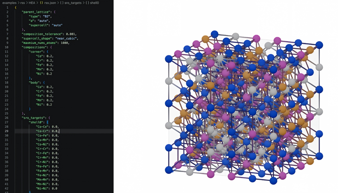
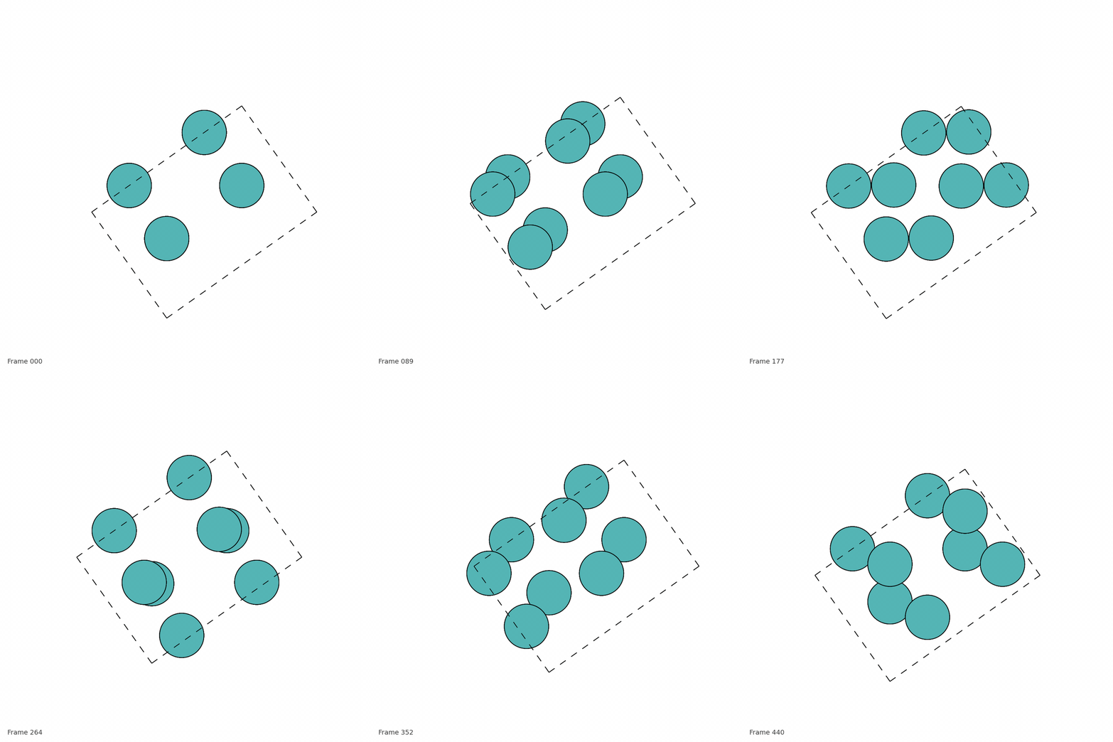
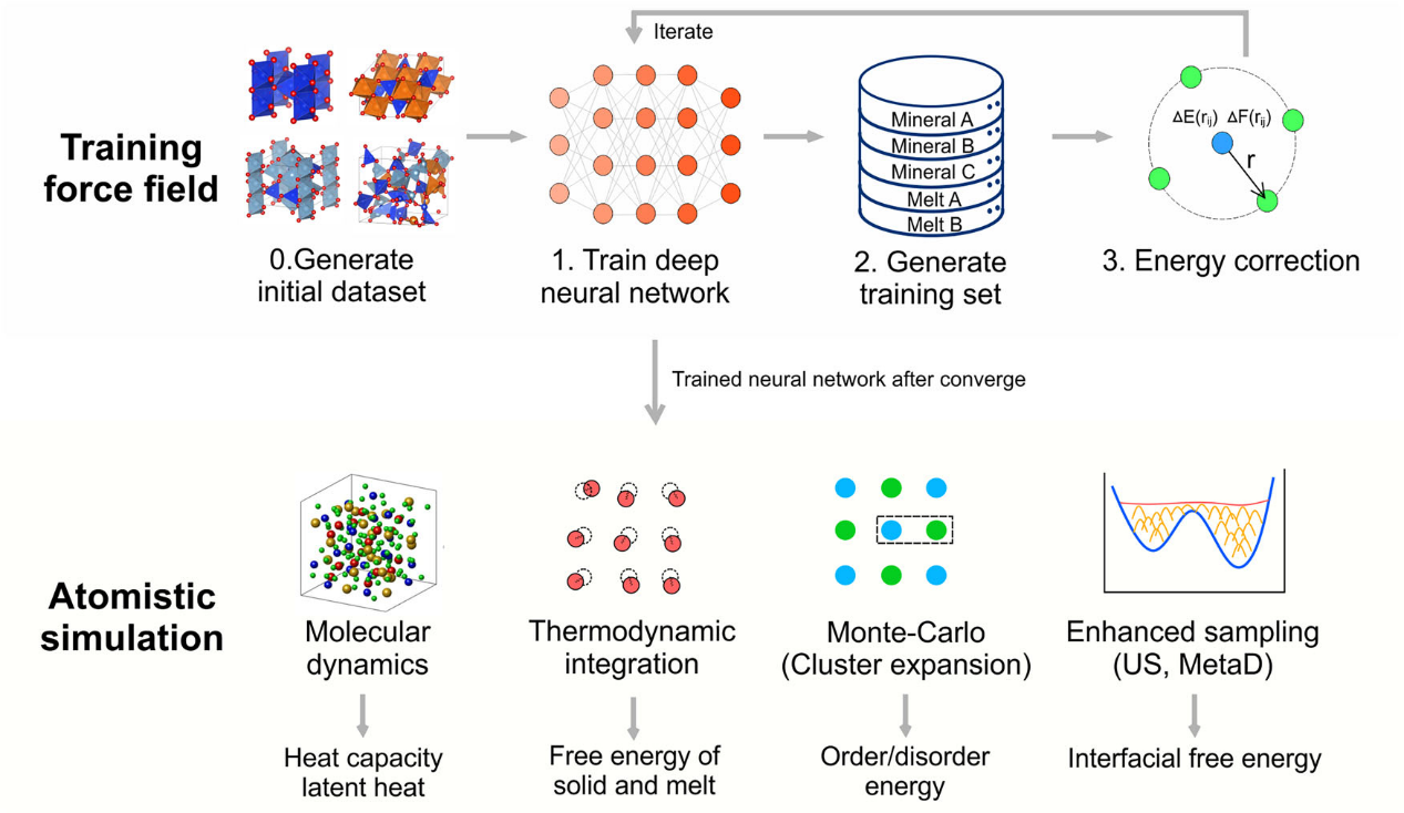
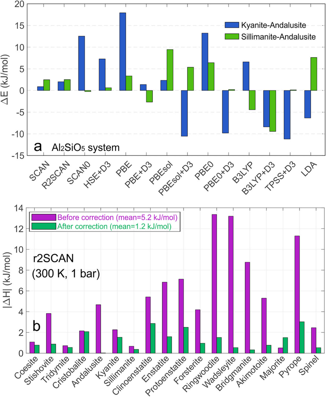
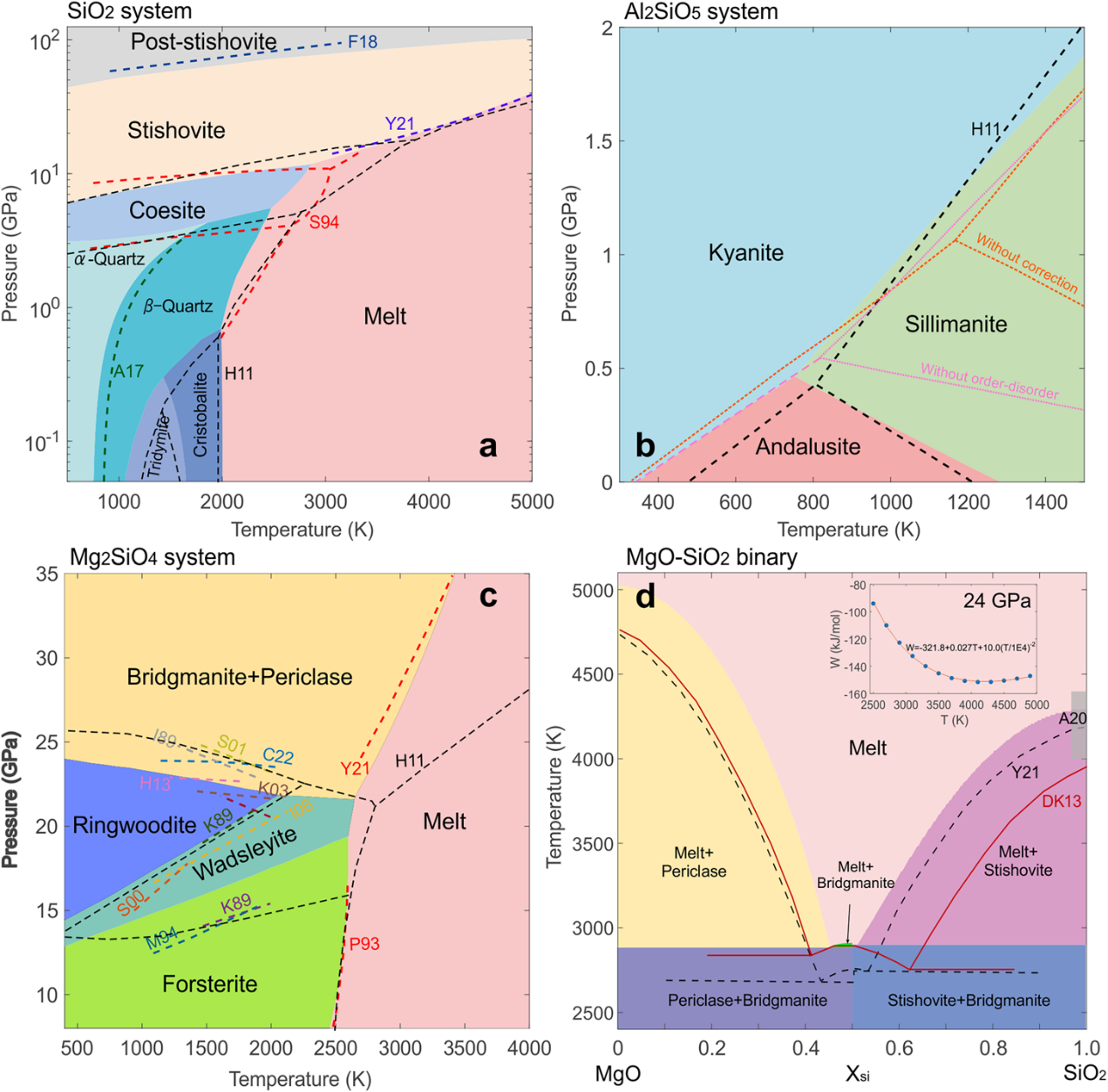
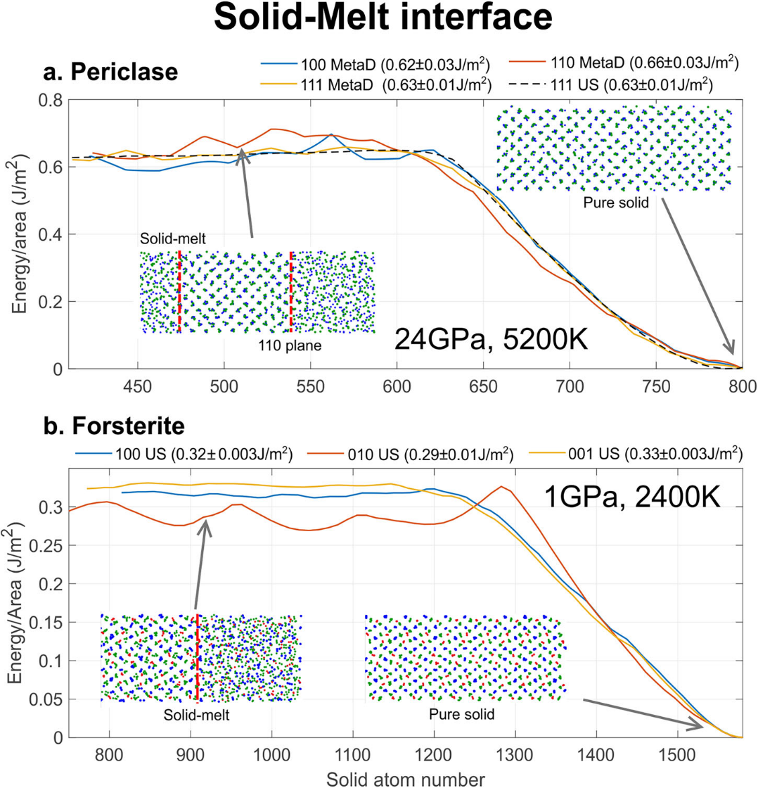
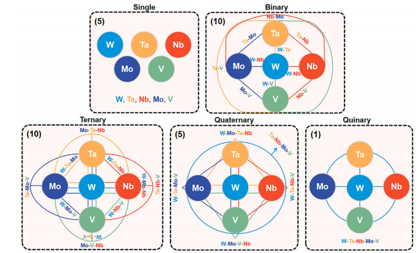
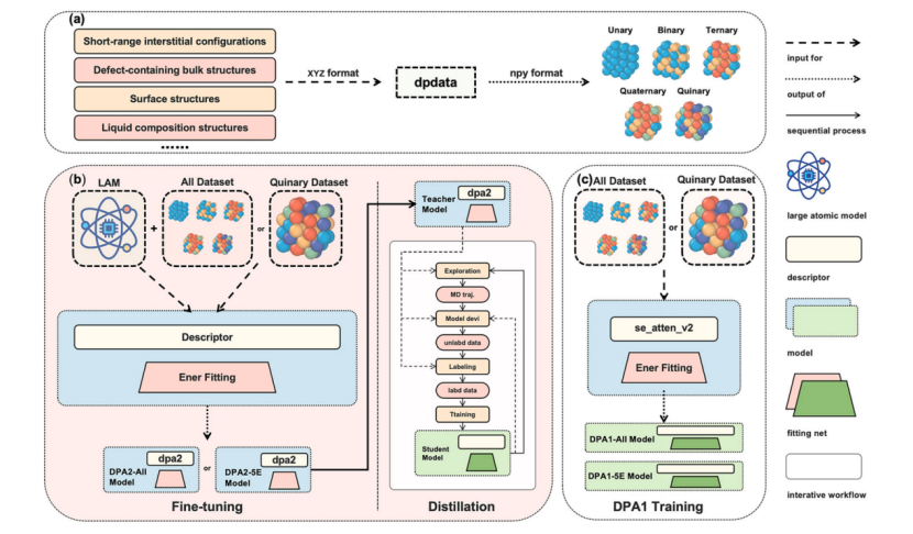
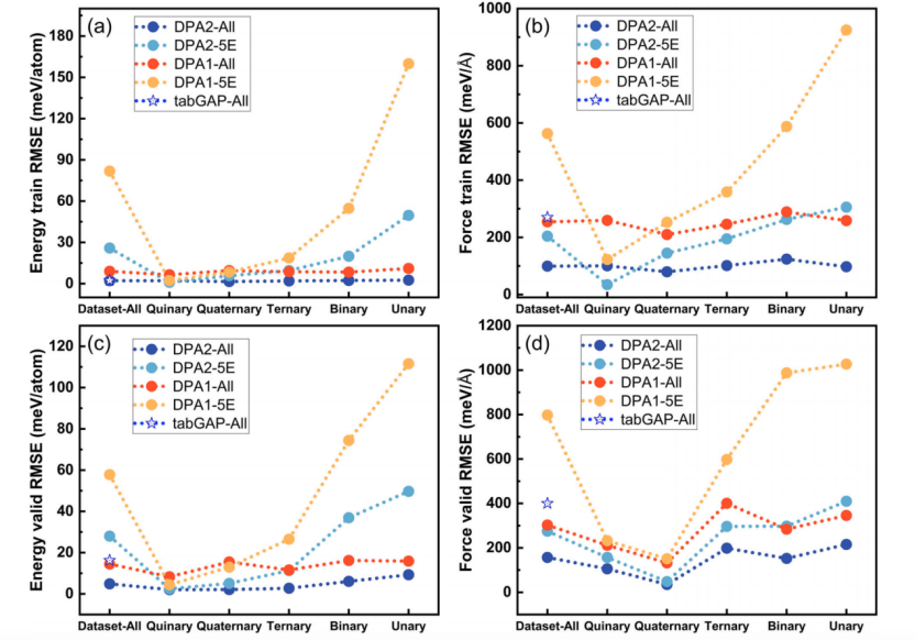
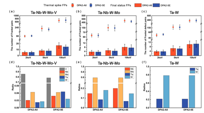
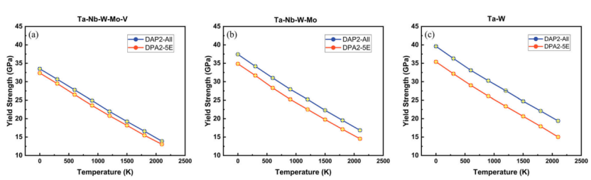
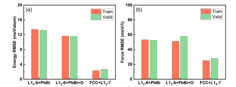
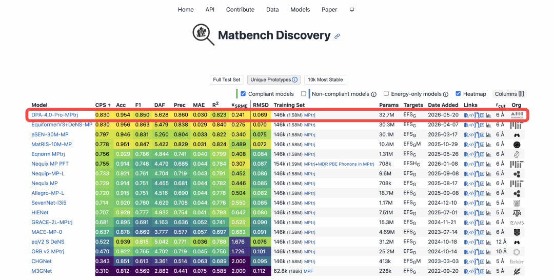
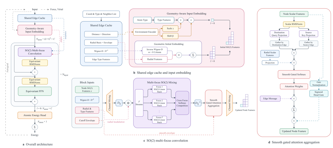
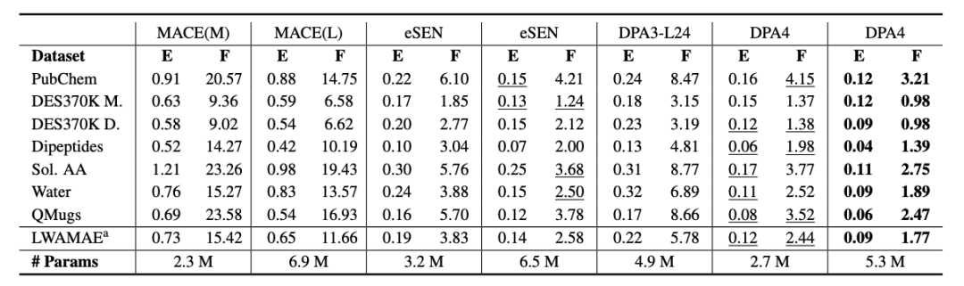
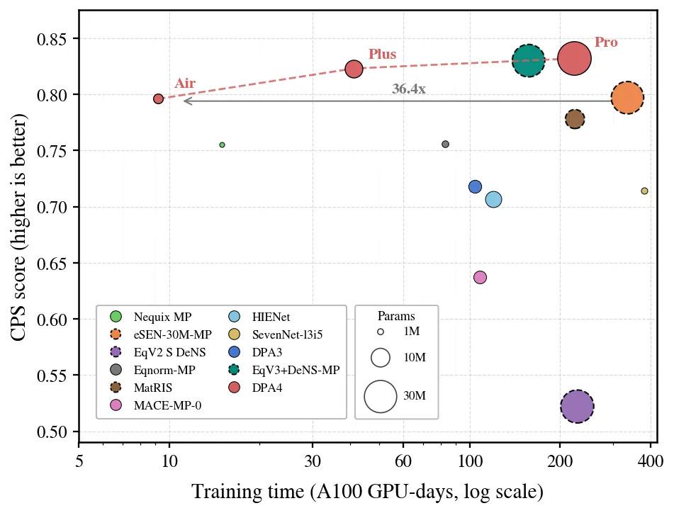
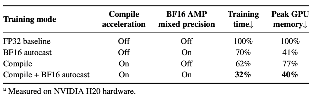
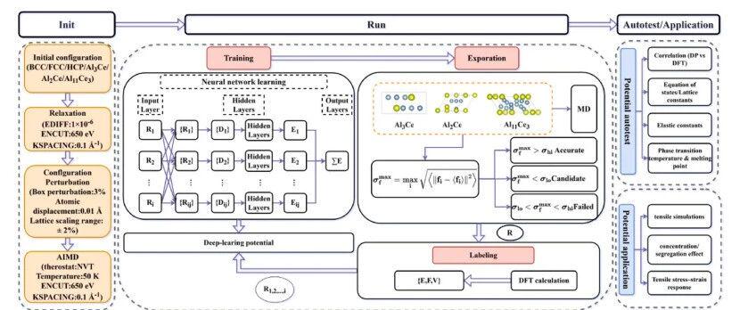
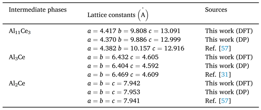
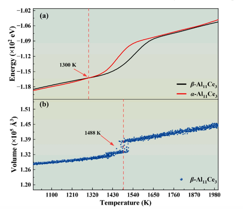
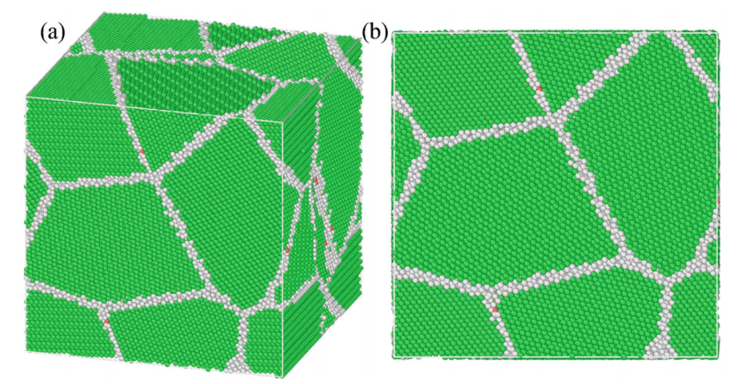
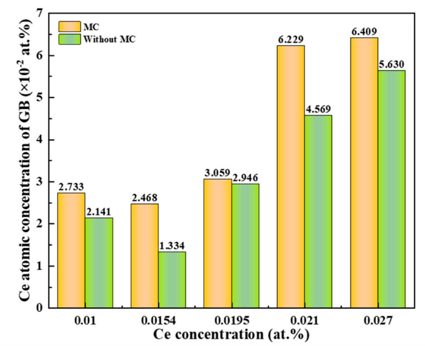
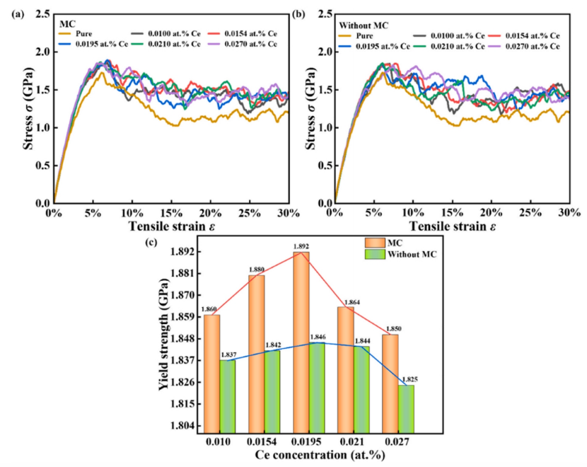
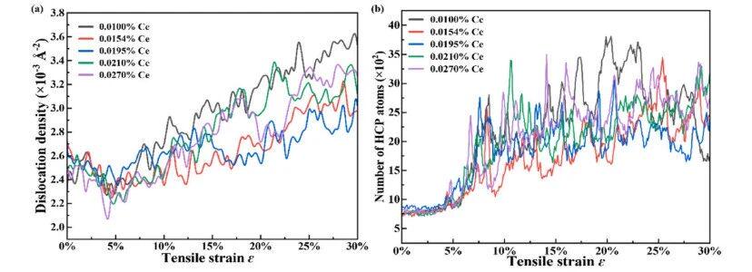
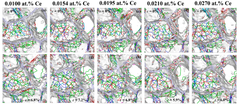
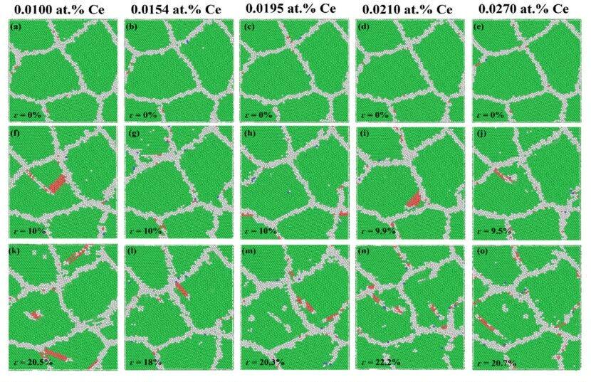
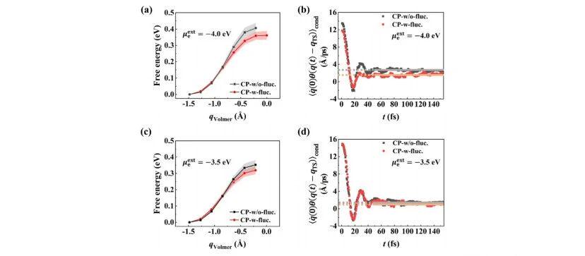
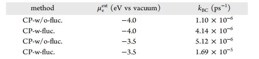
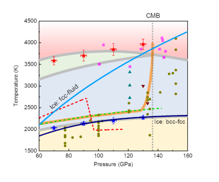
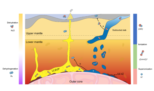
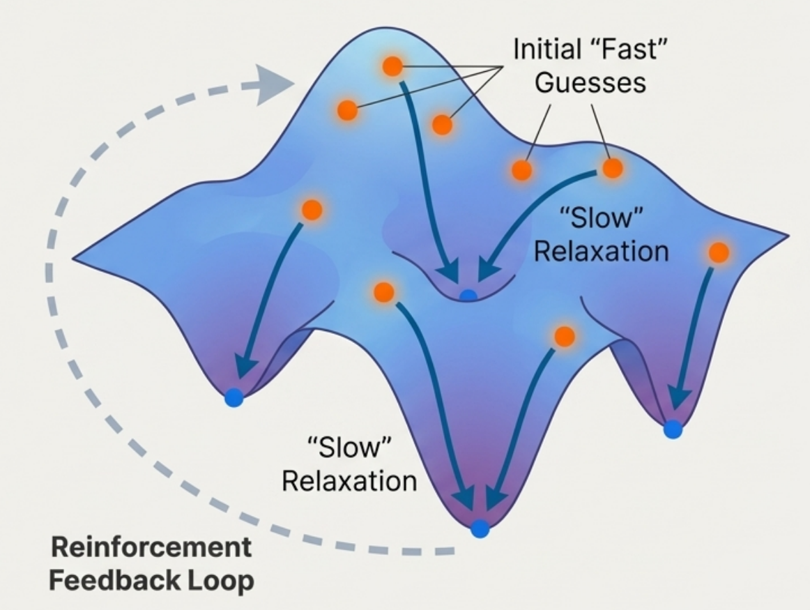
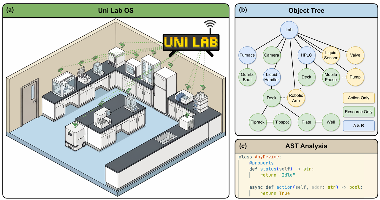
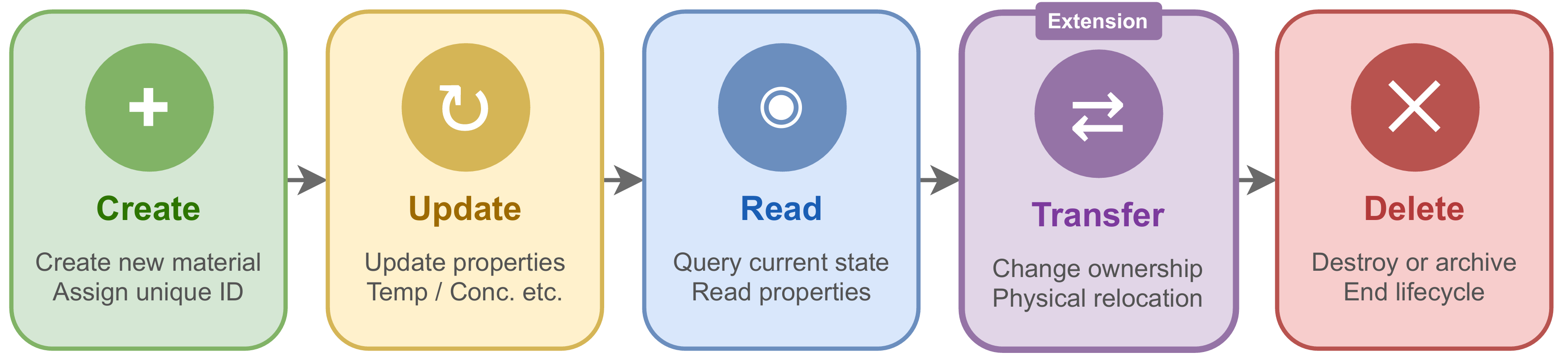
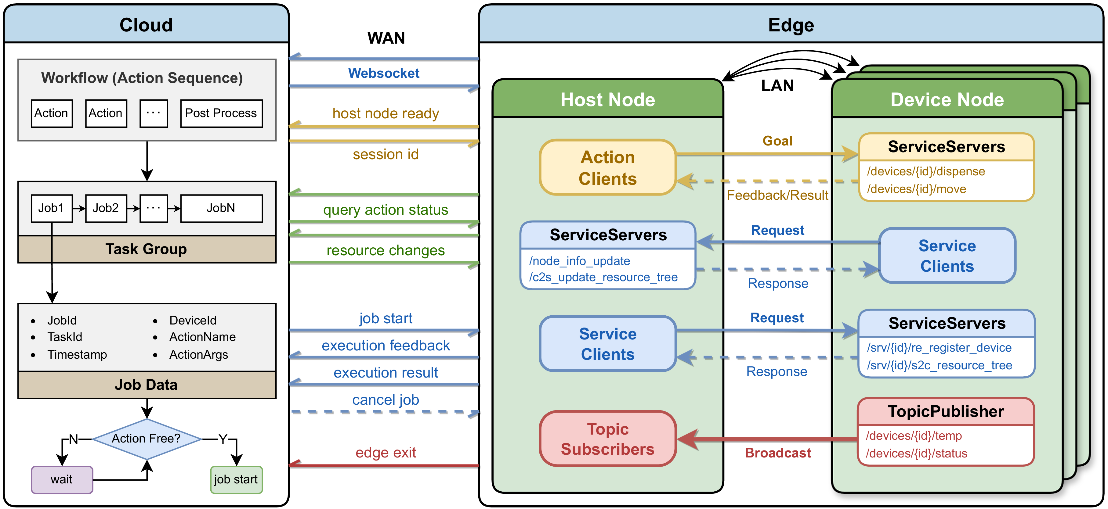
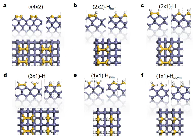
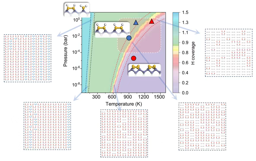
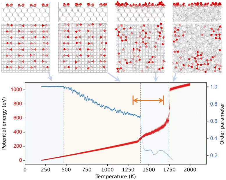
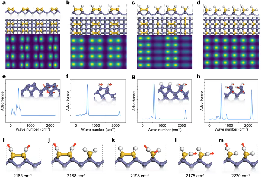
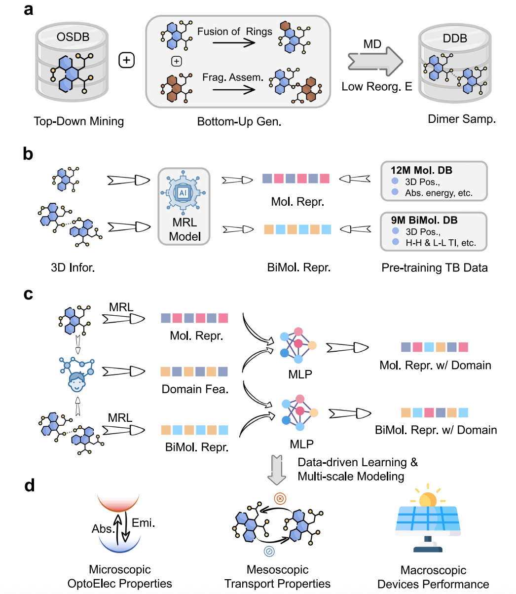
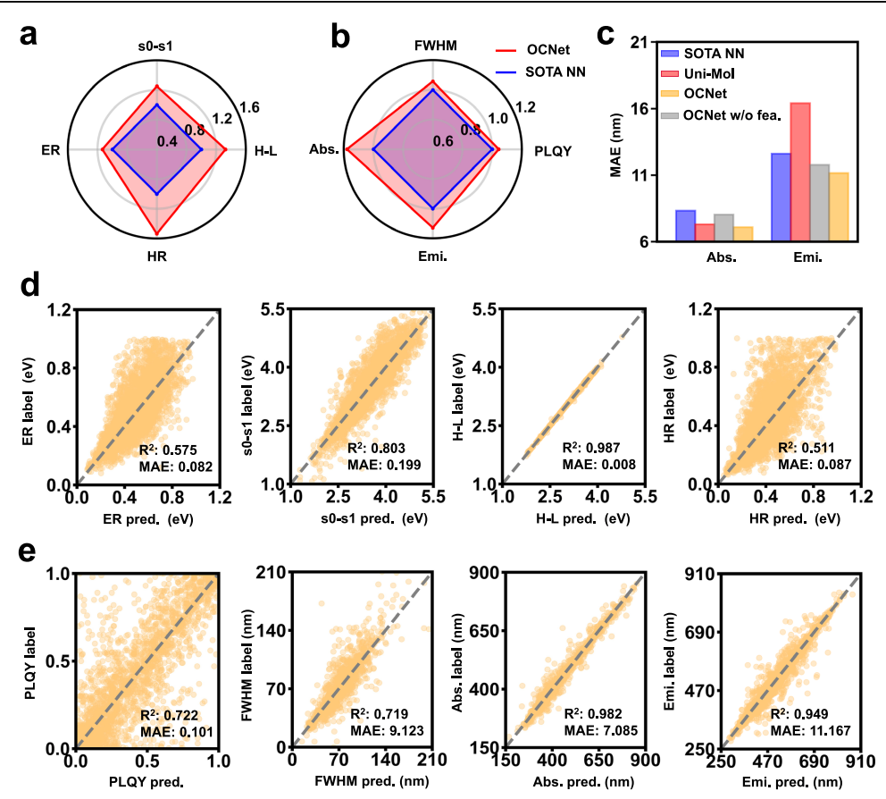
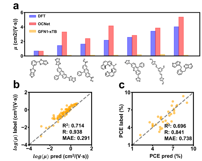
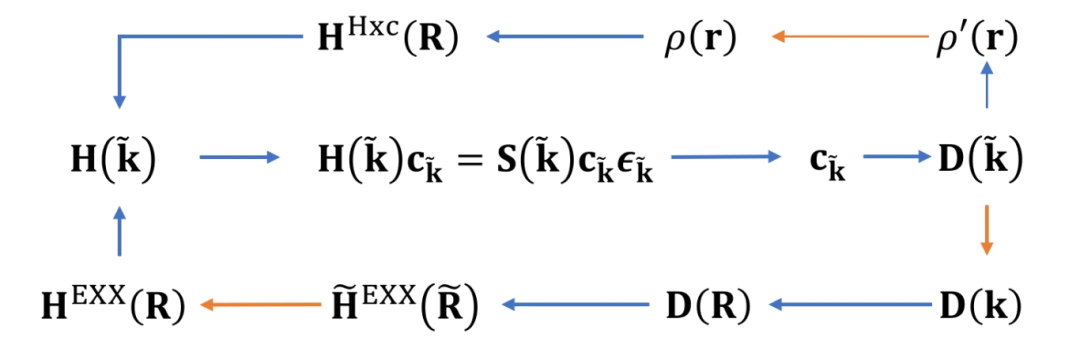
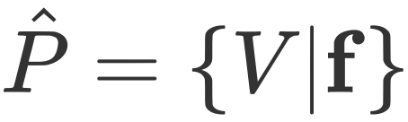 are:
are: